Manual MiXBLUP

Version 3.2.1 – 2026 – 06

MiXBLUP User’s Guide
MiXBLUP, best linear unbiased prediction (BLUP) software for PCs for large genetic evaluation systems

This manual is for MiXBLUP version 3.2, released in May 2026
MiXBLUP is developed jointly by LUKE National Resources Institute Finland and Animal Breeding & Genomics, Wageningen University & Research.

Authors:
J. ten Napel, J. Vandenplas, M. Schrauf, M.P.L. Calus, R.F. Veerkamp
M. Lidauer, I. Stranden, M. Taskinen, E. Mäntysaari

Animal Breeding & Genomics, Wageningen University & Research P.O. Box 338
6700 AH Wageningen
The Netherlands

LUKE National Resources Institute Finland
FI-31600
Jokioinen
Finland

More information on the MiXBLUP website

1. Introduction

MiXBLUP has been developed for routine breeding value estimation in commercial genetic programmes and supports modern applications, such as random regression models, group selection, the use of genetic markers or haplotypes and the use of genomic information.

1.1. Overview

The intention of developing MiXBLUP was to utilize efficient computing strategies for solving mixed model equations. With MiXBLUP it is possible to use sophisticated models in estimation of breeding values in animals, like cattle, pigs, poultry, sheep, horses, goats, dogs, and aquatic species. The software also supports many ways to specify genetic similarity between individuals, including pedigree, marker information and genomic information. The statistical method used for genetic evaluation is best linear unbiased prediction (BLUP), which is currently the common methodology for genetic evaluation.
MiXBLUP supports two solvers. The MiX99 solver has been developed for efficient use of disk space and memory. Due to iteration on data and a very fast algorithm in the solver (preconditioned conjugate gradient, PCG), it is able to solve mixed model equations very fast. It is derived from MiX99 and was initially developed for classical genetic evaluation without the use of markers or genes by LUKE National resources Institute Finland. The adaptation for the use of marker and genomic information was implemented by Wageningen UR Livestock Research in collaboration with LUKE.
The hpblup solver has been developed specifically for efficient genetic evaluation using a very large amount of genomic information. It is also based on a PCG algorithm, but genomic information is stored in memory during solving and it uses multiple cores whenever beneficial.

1.2. Manual

This manual will guide the user through the use of MiXBLUP. The examples provide a way to test the software, to get a feel for the software. A set of examples is provided as an Appendix to the manual. The number of the example refers to the corresponding chapter of this manual.
A schematic overview of the input files, output files and instruction file is in Figure 1.

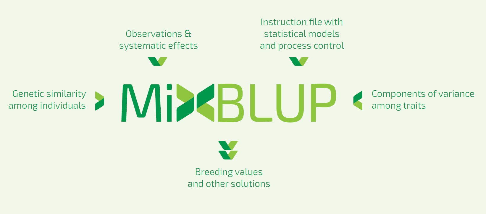
Figure 1. Schematic overview of the input and output files of MiXBLUP.

1.3. System requirements

MiXBLUP is written in standard Fortran 90 language and is self-contained. The program runs in Windows, Linux and Unix environments and is available in 64-bit version. In Windows, it runs in the command-line interpreter, cmd.exe or in the Windows PowerShell. The Windows release it is routinely tested in a Windows 11 operating system.
MiXBLUP allocates memory depending on the need. Small applications can be run with a minimum of memory available. Very large applications may need a substantial amount of memory, especially genomic analyses and the calculation of reliabilities.
MiXBLUP supports the use of multiple cores. The MiX99 solver uses all available cores for the most common genomic evaluations, only. The hpblup solver is optimised for 10-15 cores for all available types of evaluation. Preparation of data for solving and processing its results are done with a single core.

2. How to start

MiXBLUP is easy to use and easy to install. This chapter describes how to install the software and how to obtain and install a license.

2.1. Installing MiXBLUP software

Download the appropriate zip-file from http://www.MiXBLUP.eu and unzip the folder with the executables. Copy the executables to a central folder that can be accessed from other folders. The user needs to create a file, named ‘SysDir.inp’, which contains the path to the central folder with executables. This file should be copied to any folder from which MiXBLUP is run. The path to MiXBLUP.exe should be included in the command file that starts up the analysis or added to the system path. MiXBLUP uses SysDir.inp to locate the other executables.

2.2. MiXBLUP Licenses

To run MiXBLUP software on your computer you need a license. There are different license types for MiXBLUP. A license can be ordered at http://www.MiXBLUP.eu.

The license key of the commercial licenses is computer-specific. Therefore, if executables and the license key ‘LICENSE.DAT’ are moved to another computer, MiXBLUP will give an error message. Running MiXBLUP with the run-time option –D l (minus, uppercase D, lowercase L) writes the host name, license type and expiry date in the license file to the screen output. So if you want to transfer the MiXBLUP software with an existing license to a new computer, you have to request a new license from info@mixblup.eu with the LICREQST.DAT attached (how to generate a LICREQST.DAT file see below). You will receive a new license for the remainder of the license period. The license key provides the information about the MiXBLUP version, the license type and the expiry date of the license. A trial license can be used for one month and a trial license key is not computer-specific. The small and full commercial license can be used for one year. The license key for these licenses is computer-specific.

2.2.1. Trial License

Order a trial license at http://www.MiXBLUP.eu. After receiving your order, we send the necessary license key to the e-mail address in the order.

2.2.2. Commercial licenses

Order a commercial license at http://www.MiXBLUP.eu. While entering the order you are asked to upload one or more ‘LICREQST.DAT’ files. For each computer you need to upload a separate ‘LICREQST.DAT’ file. This file is required to generate a license key for your computer. Also renewing a license for the next calendar year you need to do by filling in the MiXBLUP License Order & Renewal Form on the website.

2.2.3. Generating a license-request file and installing the license

The name of the license request file is ‘LICREQST.DAT’. The name of a license file is ‘LICENSE.DAT’.

• Run MiXBLUP.exe once without the need for an instruction file. MiXBLUP creates the file LICREQST.DAT in the working directory.
  
• After payment of the license one or more ‘LICENSE.DAT’ files will be sent back and should be saved in the bin folder of the corresponding computer(s).
  
• Store the license key ‘LICENSE.DAT’ in the C:MiXBLUPbin-folder for Windows or in the /usr/bin-folder for Linux.

2.2.4. Alternative license directory

If the license key cannot be stored in the default directory, the user may create a file, named LicDir.inp, which contains the path to the license file. If this file exists, MiXBLUP will look for the license file in the specified folder.

3. Instruction file

The instruction file contains all information that MiXBLUP needs for the analysis. This chapter gives an overview of the instruction file. The various parts of the instruction file are discussed in detail in the next chapters.

3.1. Parts of the instruction file

The information in the MiXBLUP instruction file is presented in six parts. These parts are:

1. Description of the analysis
   
2. Observations & systematic effects (Chapter 4.)
   
3. Genetic similarity among individuals (Chapter 5.)
   
4. Components of variance and covariance among traits (Chapter 6.)
   
5. Statistical models (Chapter 7.)
   
6. Control of analysis and output (Chapter 8.)

These parts may be presented in the instruction file in any order. Sections within a part may also appear in any order. Below the example instruction file is given for a bivariate animal model for two traits (phen1 and phen2).

TITLE breeding value estimation for phen1 and phen2 using pedigree
# Observations & systematic effects
DATAFILE ExampleDat.txt !MISSING -99
animal A
fix1 A
fix2 I
cov R
ran A
phen1 T
phen2 T
blk I
# Genetic similarity among individuals
PEDFILE ExamplePed.txt
animal A
sire A
dam A
blkped I
# Components of variance and covariance among traits
PARFILE ExamplePar.dat
# Statistical models
MODEL
phen1 ~ fix1 cov !RANDOM ran G(animal)
phen2 ~ fix2 cov !RANDOM ran G(animal)
# Control of analysis and output
SOLVING
!MAXIT 1000
Example. Parts of the instruction file.

3.1.1. Title of the analysis

The instruction file must start with a specification of the title of the analysis. The TITLE keyword is optional. If omitted, the first line must start with a hash (#). This comment line is then used as the title of the analysis. This line can be used to describe the analysis and distinguish it from other analyses.

3.1.2. Observations & systematic effects

The data observations part of the instruction file contains the name of the files with data or covariates, their location and their record layout. The sections that can be used in this part are DATAFILE, CVRTABLE and REGFILE. The syntax of these sections, more advanced options and examples are presented in Chapter 4. of this manual.

3.1.3. Genetic similarity among individuals

Genetic similarity among individuals can be specified in many different ways. It may be based on pedigree information only, genomic information only or both sources of information simultaneously. Pedigree information may contain genetic groups for unknown parents or a single code to denote an unknown parent. Inbreeding can be taken into account or ignored. Genomic information may be incorporated through covariances between individuals or through regression on SNP covariates. Sections that can be used in this part are PEDFILE, ERMFILE, INBRFILE, SNPFILE, REGFILE, CORRFILE and CVMATRIX. The syntax of these sections and examples for the various options are presented in Chapter 5. of this manual.

3.1.4. Components of variance and covariance among traits

Genetic and non-genetic random effects have components of variance and covariance among traits in the model. Residual (co)variance components may also vary between groups of data records. Section that can be used in this part are PARFILE, RESFILE, SNPPARFILE and REGPARFILE. The syntax of these sections is presented in Chapter 6.

3.1.5. Statistical models

Statistical models are specified by trait. Each trait starts on a new line. The only sections in this part of the instruction file are MODEL, LINKEDEFFECTS and COMBINE. The syntax of the various statistical models supported by MiXBLUP are presented in Chapter 7.

3.1.6. Control of analysis and output

The control part of the instruction file can be used to specify (1) whether to solve the system (i.e. estimate breeding values) or calculate approximate reliabilities, (2) whether or not to use starting values, (3) which resources to use for parts of the process, (4) when to stop the iterative process and write out the solutions, (5) how to present the solutions, (6) which additional output files to create after the solving process has been completed and (7) how to manage temporary files. The sections that can be used in this part are SOLVING, TRAITEBV, PRECON and TMPDIR. Syntax is presented in Chapter 8.

3.2. General syntax of the instruction file

• The maximum record length of the instruction file is 5,000 characters
• The instruction file may contain empty lines for the convenience of the user
• Comments may be inserted on a new line or after instructions on the same line, provided that any comment starts with a hash (#). Any text on a line following a hash is ignored by MiXBLUP
• The keyword of any section must be the first word of the line

4. Observations & systematic effects

The data observations part of the instruction file is used to specify observed traits and any factors or covariates that cause systematic variation between observations for these traits. This chapter describes the various ways to present observations and systematic effects.

4.1. Data file

4.1.1. General

Observations and systematic effects are normally presented in the data file. All traits and effects in the statistical model must have a column in the data file, except for covariates in a covariate table file and covariates in an external covariate file. The name of the data file is specified in the instruction file. The data file is located by default in the work directory, but it can be in any other folder if this is specified as part of the name of the file (e.g. d:PerformanceTestBreedP.txt). The order of the fields in the DATAFILE section must be the same as the order of the fields in the data file.

4.1.2. Input file

The data fields (individuals, systematic effects and trait observations) each have their own column in the data file. The data file must be provided in space-separated format, which means that any two columns are separated by at least one space. Data fields can be integer values or alphanumeric labels for class effects or real values for covariates and trait observations. Real values are read with a decimal point.

Details of the layout of the data file:

• The maximum column width in the data file is 25 characters.
• The maximum record length of the data file is 5,000 characters.
• When data is alphanumeric, any of the symbols on the keyboard can be used, including a slash (‘/’).
• An alphanumeric string must not contain spaces or it will be interpreted as two strings.

• For the MiX99 solver, a class effect must not be zero or negative if it is a number, regardless of whether it is declared as integer or alphanumerical. Data records with a class effect in the model that is zero are omitted from the analysis by the kernel as invalid data points. Therefore, MiXBLUP replaces any classes of zero or a negative number with a 1 for an integer class effect or “NA” for an alphanumerical class effect. This will not affect the results of the evaluation if the invalid classes are not associated with a valid trait observation. It is left to the user to verify that this is indeed the case.

• The default missing-value indicator for traits and covariates is zero. Data records with a covariate in the model that is equal to the missing-value indicator are omitted from the analysis by the kernel. If zero is a valid level for one of the covariates in the model, another missing-value indicator should be used. The missing value indicator has to be numerical.

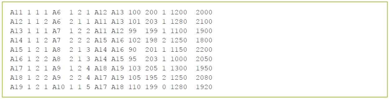
Example. Columns in data file: animal ID, mean, herd, sex, dam ID, haplotype 1, haplotype 2, common environment, pen mate 1, pen mate 2, age 1, age 2, genotype, body weight at age 1, bodyweight at age 2.

4.1.3. Syntax

DATAFILE <filename> [!SKIP <n lines>] [!MISSING <value>] [!SLASH] [!STATS [N][D][H][L]] !MINMAX <filename>
<field 1> <field type: I/R/T/A>
...
[<field i> I !BLOCK]
[<field j> I !RESVARCLASS]
...
[<field n>] [I/R/T/A]

Section:

DATAFILE
The DATAFILE section contains all the details of the file with trait observations and systematic effects.

Qualifiers:

!MISSING <value>
If the value specified for !MISSING is encountered when reading traits or covariates in the data file, it is interpreted as a missing observation for that trait or covariate. A missing covariate invalidates the trait for which the covariate is included in the model.

!BLOCK
This field is used as the block variable. If used, the data file and pedigree file both need to contain this column. It is required for the calculation of reliabilities, but might be beneficial in some computationally heavy genetic evaluations. The field must be integer. The !block qualifier must not be specified in the PEDFILE section, but the fourth column in the pedigree file must have the same field name as the block variable in the data file.

!RESVARCLASS
This field is used to specify the residual variance class of the data record, in case the residual variance differs for groups of records. The field must be integer. The qualifier !RESVARCLASS must be used if the section RESFILE is specified.

!SKIP <value>
With this qualifier, one (!SKIP 1) or more (e.g. !SKIP 2) header lines in a data file can be ignored when reading the data file.

!SLASH
The qualifier !SLASH is optional and is used when any of the input files contains a forward slash (‘/’) as a character. A forward slash is also a control character in certain file formats. If !SLASH is not specified, but MiXBLUP encounters a record with a forward slash, it will re-start reading the file as if !SLASH had been specified. Reading of data with !SLASH specified is slower than normal reading of data.

!STATS NDHL
The qualifier !STATS can be used to obtain a summary of descriptive statistics of files in the evaluation, written to Statistics.log. There are four types of statistics that can be produced: N for numbers of records in data, pedigree and genotype file; D for means and standard deviations of traits and covariates in the data; H for grouping class effect levels for each trait by the number of records per class and L for a table by trait with number of records for each class effect level. For large evaluations, it is recommended to use !STATS NDH, as the option L might produce a very large output file. Types may be specified in any order. If D, H or L are specified, N is automatically included.

!MINMAX <filename>
The qualifier !MINMAX can be used to specify a file with the valid ranges of traits and covariates. The file contains three fields for each record: the name of the field in the data file (case-sensitive!), the minimum and the maximum valid value. Field records may be in any order and may contain field records of other data files, like the parameter file.

More details of the syntax of the DATAFILE section:

• The field specification must start on the line following the line containing the DATAFILE keyword
• The field type indicates whether a field in the data file should be read as an integer value (I), a real value for covariates (R), a real value for a trait (T) or a text string (A).
• Maximum length of field names is 8 characters. A field name may be up to 19 characters long, but only the first 8 characters are used to distinguish fields, so a warning is given to remind the user.
• Field names longer than 19 characters result in an error.
• Field names are case-sensitive.
• The qualifier !BLOCK only affects the MiX99 solver. If it is specified for multiple data fields, only the first specification is used.
• Alphanumerical labels of a class effect (fields coded with A) are converted into integer values for the analysis. Solutions are decoded back to the original alphanumerical labels of the effect.
• Each alphanumerical label in a field in the data file gets a unique numerical value. There is no apparent relation between the alphanumerical label and numerical value, so the numerical value of a string may vary across runs without using old solutions as starting values. The numerical value of a string does not change if old solutions are used as starting values by specifying !RESTART in the SOLVING section.
• When using the hpblup solver, there is effectively no difference between field types A and I, as both types will be treated as alphanumeric.
• The ID of animal in the data file, and the IDs of animal, its sire and its dam in the pedigree file must all be of the same type, so either alphanumeric (A) or numeric (I).
• The largest integer number that can be used as level of a class effect is approximately 2,100,000,000 (2^31^). For class effects with levels that exceed this number, the field type has to be set to alphanumerical (A).

• The version of the data file with alphanumerical labels converted to integer values is ‘data.txt’ for the MiX99 solver and hpData.txt for the hpblup solver.

• The use of names reserved as section keywords, qualifiers or functions as field names is not supported.

4.1.4. Associated output files

Output file	Description
data.txt	temporary file; data file prepared for analysis by kernel

4.2. Covariate table file

4.2.1. General

If the relationship between an independent variable and a dependent trait is modelled as an n^th^ order polynomial, a covariate table file with all levels of the independent variable between its minimum and maximum value in the data and (n+1) columns of covariates may be used for easy presentation of covariates and syntax of the instruction file. The name of a pre-defined covariate table file is specified in the instruction file. The name may include the path to the covariate table file. A covariate table file can also be created in MiXBLUP. Currently only a Legendre polynomial is supported. A covariate table is created using the minimum and maximum value of the independent variable and the required order of the polynomial. The minimum and maximum value of the independent variable can either be specified by the user or determined from the data. For the MiX99 solver, only one covariate table can be used, but its columns may be fitted within multiple class effects. Additional polynomials using other independent variables should be added as columns in the data file prior to calling MiXBLUP. For the hpblup solver, it is possible to use multiple covariate table files and indices to link covariate records to data records may be different between covariate tables.

4.2.2. Input file

A covariate table file may be created outside of MiXBLUP, it may have been created in a previous analysis or it may be created at run-time. It consists of the original independent variable and the n+1 covariates derived from it, with n being the order of the polynomial. If the order is n, the covariate columns in the table are numbered from 0 to n, giving n+1 covariate columns in addition to the original independent variable. The independent variable has to have an integer field type. The covariate table should contain all levels between the minimum and maximum value with steps of one. It means that an independent variable with decimals must be converted to integer values before a covariate table can be used for it. The independent variable links the record in the data file with the covariate record in the covariate table. The column in the data file with the independent variable must contain a valid entry for every record. For the hpblup solver, each covariate table must have a unique label that starts with TABLE followed by a number between 01 and 99.

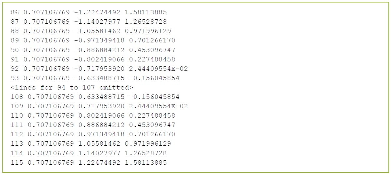
Example. A covariate table file for an independent variable with values in the data between 86 and 115. The order of the Legendre polynomial is 2. The table was created with the line !CVRMAKE LEG !CVRNUM 2 !CVRMIN 86 !CVRMAX 115 in the CVRTABLE section of the instruction file.

4.2.2.1. Syntax using an existing covariate table for the MiX99 solver

DATAFILE <filename>
...
<field k> I !CVRIND
...
CVRTABLE <filename>
MODEL
<trait> ~ <fixed effects> <Class1>*CVR(n1) !RANDOM <Class2>*CVR(n2) G(Animal*CVR(n3))
...

Sections:

CVRTABLE/ The CVRTABLE section contains the details of the existing or new covariate table.

Qualifiers:

!CVRIND / The field marked with !CVRIND is the independent variable used in polynomial regression. Any level of the field specified with !CVRIND must exist in the covariate table file. The field must not contain a missing value indicator for a valid trait observation. The qualifier !CVRIND must be used when the section CVRTABLE is specified. The field must be integer. The qualifier !CVRIND, specified in DATAFILE section, should not be confused with !CVRindex that is used with hpblup solver and specified in the CVRTABLE section.

CVR(...) / The CVR function is used in the MODEL section and is a shorthand for all polynomial terms to be fitted and may be used in the same way as any individual random regression term. The alternative way to specify polynomial random regression is to use the individual columns of the covariate table file. The names of the columns are cvr00, cvr01, cvr02, ..., cvrnn.

4.2.2.2. Syntax using an existing covariate table for the hpblup solver

...
CVRTABLE !nCVRTABLES 2
TABLE01 <filename> !CVRNUM <n^th^ order> !CVRMIN <minimum value> !CVRMAX <maximum value> !CVRSingleCov !CVRIndex <index field name>
TABLE04 <filename> !CVRNUM <n^th^ order> !CVRMIN <minimum value> !CVRMAX <maximum value> !CVRSingleCov !CVRIndex <index field name>

MODEL
<trait> ~ <fixed effects> <Class1>*TABLE01 !RANDOM <Class2>*TABLE04 G(Animal*TABLE04)
...

Additional qualifiers:

!nCVRTABLES
This qualifier specifies the number of covariate tables included in this section

!CVRIndex
This qualifier specifies the field name of the index in the DATAFILE. Please note that this option is different from !CVRIND, which is used with the MiX99 solver and specified in the DATAFILE section.

!CVRSingleCov
This qualifier is used to create a separate file for each covariate in table specified. Each covariate in the table is then be fitted as a separate effect for the hpblup solver.

TABLEtt in the MODEL section
A covariate table file specified in the CVRTABLE section can be fitted in the model by fitting its label. It may be used in the same way as any individual random regression term. The names of its columns in variance covariance matrix files are cvrtt_00 to cvrtt_nn, where tt is the number in the label of the covariate table and nn the order of the polynomial specified for the covariate table tt.

4.2.2.3. Syntax using a newly created covariate table for the MiX99 solver

DATAFILE <filename>
...
<field k> I !CVRIND
...
CVRTABLE !CVRMAKE LEG !CVRNUM <n^th^ order> !CVRMIN <minimum value> !CVRMAX <maximum value>
MODEL <trait> ~ <fixed effects> <Class1>*CVR(n1) !RANDOM <Class2>*CVR(n2) G(Animal*CVR(n3))
...

Additional qualifiers:

!CVRMAKE
If !CVRMAKE is specified, MiXBLUP generates a covariate table file using the settings specified with the !CVRNUM, !CVRMIN and !CVRMAX qualifiers. Currently, only a covariate table containing Legendre polynomials can be created, by specifying LEG as the argument of !CVRMAKE. The name of the new covariate table file is ‘cvrtable.txt’.

!CVRNUM
The qualifier !CVRNUM must be specified and is used to specify the order of the polynomial in the covariate table. The expected number of columns to read is the order + 2, one for the level of the independent variable and one for the order being 0. It is up to the user to make sure that the order specified in the MODEL section is equal to or lower than the order specified with !CVRNUM.

!CVRMIN and !CVRMAX
The qualifiers !CVRMIN and !CVRMAX can be used to specify the lowest and highest value of the independent variable that were used to estimate the genetic parameters. Legendre polynomials are dependent on the lowest and highest value of the independent variable and so are the genetic parameters of Legendre polynomials. If !CVRMIN or !CVRMAX is nevertheless omitted, the lowest or highest value of the independent variable in the data is used, instead.

4.2.2.4. Syntax using newly created covariate tables for the hpblup solver

...
CVRTABLE !nCVRTables <value>
TABLE01 !CVRMAKE LEG !CVRSingleCov !CVRNUM <n^th^ order> !CVRMIN <minimum value> !CVRMAX <maximum value> !CVRIndex <field name of the index>
TABLE02 !CVRMAKE LEG !CVRNUM <n^th^ order> !CVRMIN <minimum value> !CVRMAX <maximum value> !CVRIndex <field name of the index>
...
MODEL <trait> ~ <fixed effects> TABLE01 !RANDOM <Class>*TABLE02 G(TABLE02*animal)

Additional qualifiers:

!CVRMAKE
If !CVRMAKE is specified, MiXBLUP generates a covariate table file using the settings specified with the !CVRNUM, !CVRMIN and !CVRMAX qualifiers. Currently, only a covariate table containing Legendre polynomials can be created, by specifying LEG as the argument of !CVRMAKE. The name of the new covariate table file is ‘hpTablett.txt’, for example hpTable01.txt. If !CVRSingleCov is specified, a separate file is created for each covariate. In that case, the names of the new covariate table files are ‘hpTablett_nn.txt’, for example hpTable01_00.txt, where tt is the number in the label of the covariate table and nn the number of the covariate of the polynomial specified for the covariate table tt, ranging from 0 to the order specified.

4.2.3. Associated output files

Output file	Description
cvrtable.txt	covariate table, if created by MiXBLUP

4.3. General covariate files

4.3.1. General

Some covariates are individual-specific: they never change for an individual, but vary across individuals. They are more associated with the individual than with its data records. Examples are breed composition, genetic groups, heterosis and recombination. Such covariates can be stored in a covariate file, in which all individuals in the analysis have a record. MiXBLUP converts the covariate file with all individuals to a data covariate file that exactly matches the data file, including repeated records.

4.3.2. Input file

General covariate files contain at least the ID of the animal and any number of covariates, but all records should have the same number of covariates. General covariate files must be provided in space-separated format. Covariates are read as real numbers, regardless of whether a decimal point is present in the corresponding field. General covariate files contain at least all individuals with a phenotype for any of the traits in the statistical model. Individuals without any phenotypes will be ignored, except in the case of genetic group covariates.

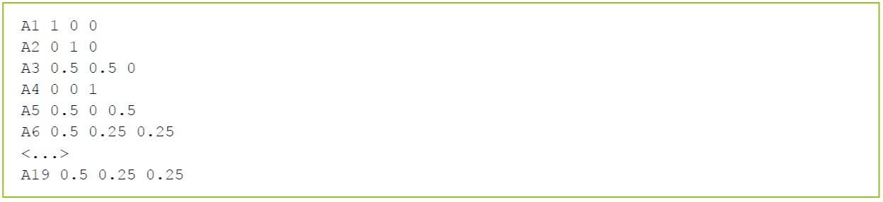
Example. Covariate file with breed fractions in a mixed breed population

4.3.3. Syntax

4.3.3.1. Syntax of a general covariate file and associated variance-covariance file

REGFILE
<field animal> <field type I or A>
REG01 <file name REG01> !REGTYPE F/R/H [!IDCOL 1] [!STARTCOV 2] [!LASTCOV 7]
REG02 <file name REG02> !REGTYPE F/R/H [!IDCOL 1] [!STARTCOV 2] [!LASTCOV 7]
...
REG99 <file name REG99> !REGTYPE F/R/H [!IDCOL 1] [!STARTCOV 2] [!LASTCOV 7]

REGPARFILE
REG01 <file name REG01>
REG02 <file name REG02>
...
REG99 <file name REG99>

Sections:

REGFILE
The REGFILE section specifies the name of one or more general covariate files and its attributes, such as column numbers and whether one variance for all covariates is used or an individual variance for each covariate.

REGPARFILE
The REGPARFILE section is used to specify a file with components of variance and covariance among traits associated with general covariates. A general covariate file labelled in REGFILE needs a corresponding entry in a REGPARFILE section if the regression type is R for random or H for heterogeneous variances. There are no file-independent qualifiers.

Qualifiers:

The file-dependent qualifiers of REGFILE can be specified for each covariate file. These qualifiers are explained below.

!REGTYPE
The file-specification line must contain the !REGTYPE qualifier. It specifies how the covariates in the file are fitted in the model. If ‘f’ is specified, the covariates in the file are fitted as a fixed regression. Covariates fitted as a fixed effect do not have a variance associated with it, so it is not necessary to specify a parameter file in the REGPARFILE section. If it is present, it is ignored. If ‘r’ is specified, the covariates in the file are fitted as a random regression with a single variance for all covariates in the file. The variance is specified in the corresponding parameter file in the REGPARFILE section. If ‘h’ is specified, the covariates in the file are fitted as a random regression, each with their own variance. The covariate-specific variances are specified in the corresponding parameter file in the REGPARFILE section.

!IDCOL
The !IDCOL qualifier is optional and specifies which field in the covariate file contains the ID of the individual. If it is omitted, it is assumed that the ID is in the first field of the record (so the default is !IDCOL 1).

!STARTCOV
The !STARTCOV qualifier is optional and specifies which field contains the first covariate. If it is omitted, it is assumed that the covariates start in the second field of the record (so !STARTCOV 2).

!LASTCOV
The !LASTCOV qualifier is optional and specifies which field contains the last covariate of the file to include in the model. If it is omitted, it is assumed that all fields after the first covariate contain covariates to include in the model.

4.3.3.2. Syntax of fitting a general covariate file in the model for the MiX99 solver

MODEL trait ~ fixed !RANDOM REG(1,2..5)

Qualifiers:

REG(...)
The REG function is used in the MODEL section and can be used to specify which general covariate files should be fitted in the model of a trait. If a covariate file is specified, then all specified covariates in the file will be fitted simultaneously. The numbers in the REG(...) function link to the number in the label of the general covariate file in the REGFILE section (and the REGPARFILE section). The numbers may be specified individually as (1, 2, 3, 4) or as a range, indicated by two subsequent full stops, for example (1..4), or a combination of both. If a covariate file is fitted for any trait through REG(...), the covariates will be fitted for all traits, even the ones for which REG(...) is not specified.

4.3.3.3. Syntax of fitting a general covariate file in the model for the hpblup solver

MODEL trait ~ <fixed> !RANDOM hpREG(1,<field index>)

Qualifiers:

hpREG(<number in label of covariate file>, <field index>)
The hpReg function is used to fit a general covariate file in the model of a trait, for which it is specified. For a random effect, REGTYPE needs to be set to R or H and hpREG needs to be specified after the !Random qualifier. For a fixed effect, REGTYPE needs to be set to F and hpREG needs to be specified before the !Random qualifier.

4.3.4. Associated output files

Output file	Description
RegCov%%.txt	temporary file; data covariate file
RegCov%%NoDat.txt	temporary file; covariates of individuals without any phenotypes
Solreg_mat.txt	solutions of all covariates in any general or SNP covariate file

4.4. Random effects with correlated level effects

4.4.1. General

For non-genetic random effects, it is often assumed that level effects are uncorrelated. In practice, this may not be a valid assumption, for example for subsequent year-seasons within a herd. For these cases, the user may provide a correlation matrix to model that some level effects are more similar than others.

4.4.2. Input file

The inverse of the correlation matrix has to be provided as a sparse matrix in I-J-Value format. The file contains a line for each non-zero element in the matrix. The line contains effect label of row, effect label of column, non-zero element. It has to be provided in upper-triangular format, so I is equal to or lower than J in the I-J-Value format. The user has to verify that the inverse correlation matrix is positive definite and not close to singularity.

4.5. Syntax

CORRFILE
RCE01 <file name RCE01>
RCE05 <file name RCE05>

MODEL
<trait> ~ <fixed> !RANDOM RCE(<random effect name for RCE01>,1) RCE(<random effect name for RCE05>,5) G(…)

Sections:

CORRFILE
The CORRFILE section specifies the name of one or more inverse correlation matrix files for non-genetic random correlated effects. The CORRFILE section does not have qualifiers for non-genetic random effects. For use of CORRFILE for specifying additional genetic relationship matrices.

4.5.1. Associated output files

Output files are the same as for non-genetic random uncorrelated effects.

5. Genetic similarity among individuals

Two individuals that have an ancestor in common are more similar than two unrelated individuals. This genetic similarity can be specified in various ways. This chapter describes the recommended methods in MiXBLUP to specify genetic similarity.

Chapter 5.1. describes the format of pedigree information that is used to build A^-1^. If only a pedigree is available, MiXBLUP will calculate the expected genetic relationships between individuals as they appear in the inverse pedigree relationship matrix (A^-1^), without the need to specify this matrix explicitly (chapter 5.3.).
Chapter 5.2. describes the recommended format of genomic data. If all or part of the individuals were genotyped for many genetic markers, such as SNPs, MiXBLUP can be used to estimate true genetic similarity from genomic data (chapter 5.4.). One method is to calculate the estimated true genetic relationships in a genomic relationship matrix. This inverse genomic relationship matrix can be used on its own if no pedigree information is available (chapter 5.4.1.2.). It can also be combined with pedigree information to analyse genotyped and non-genotyped individuals simultaneously (chapter 5.4.2.2.). Pedigree information can also be used if all individuals are genotyped.
An equivalent method to use estimated true genetic relationships implicitly, without the need to construct and invert a genomic relationship matrix, is random regression of all SNPs simultaneously on the data (chapter 5.4.1.3. and chapter 5.4.1.4.) and 5.4.2.4.).
Genetic similarity in case of multiple breeds and crosses can be addressed with breed-specific allele frequencies, breed-specific genetic groups or a fixed effect of breed composition in the model (chapter 5.6.)
It can be necessary to provide an existing inverse relationship matrix if, for example, the Henderson rules to calculate the inverse pedigree relationship matrix directly do not apply. MiXBLUP will use this matrix to model genetic similarity between individuals (chapter 5.5.). The G(...) function and the SNP(...) or hpSNP(...) functions in the MODEL section are used to link genetic similarity to data records (Chapter 7.).

5.1. Preparing pedigree data

5.1.1. General

Expected genetic similarity between individuals can be based on observed pedigree relationships. Any individual occurring in the data file, regardless of whether it occurs with a record or as a maternal, paternal or group mate genetic effect (in case of a social interaction model), must be present in the pedigree file. Any individual that does not appear in the data file, but exists as an ancestor in the pedigree file, must also have its own record in the pedigree file.

5.1.2. Recommended file formats

5.1.2.1. Pedigree file

The pedigree file consists of the individual identification code (ID) and the IDs of its sire and dam in the first three columns. The columns must be separated by at least one space. The IDs in the pedigree file must be of same type as the IDs in the data file (either numeric or text). The pedigree file may contain other information in any number of additional columns, as long as the number of columns is the same for all records.
Calculating reliabilities requires a block variable to be present in the pedigree file (see Chapter 9.). In that case the pedigree file, as well as the data file, will be sorted on the block variable. If a block group variable is added to the pedigree, it must be marked with the qualifier !BLOCK. It does not have to be in the fourth column, as in older versions of MiXBLUP. The pedigree file does not need to be sorted. MiXBLUP takes care of any required sorting.

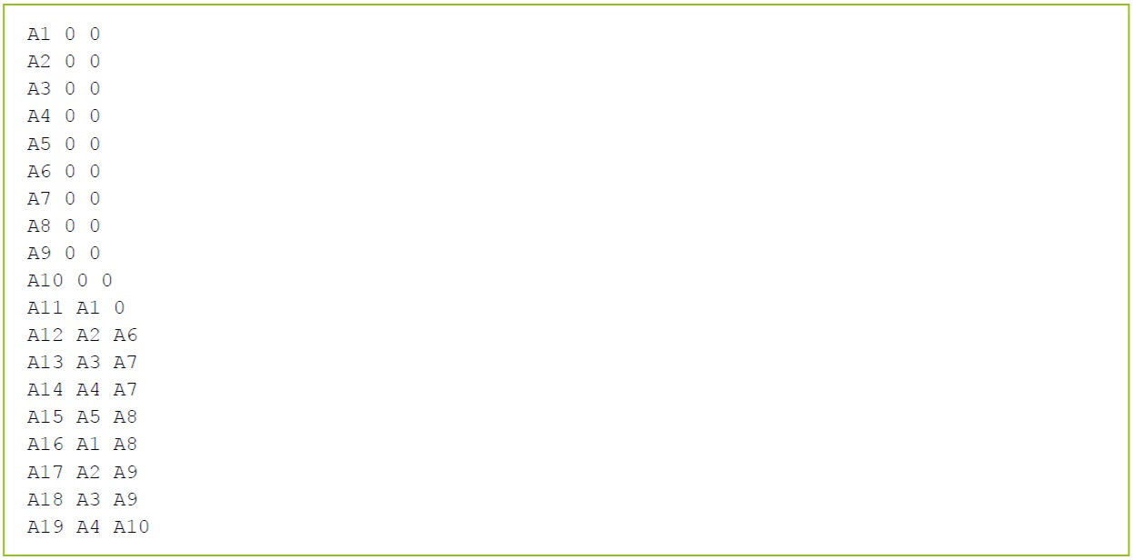
Example. Pedigree file with a single code for unknown parents/

5.1.2.2. Pedigree inbreeding coefficient file

A file with previously calculated pedigree inbreeding coefficients can be any free-format text file with any number of columns, as long as it contains the ID of each individual in the analysis and its inbreeding coefficient. This may be the pedigree file with an additional column of inbreeding coefficients.

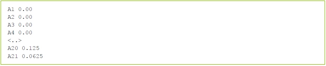
Example. File with inbreeding coefficients

5.1.3. Pedigree inbreeding coefficients

5.1.3.1. General

Inbreeding coefficients are often ignored in breeding value estimation using pedigree relationships only. The internally calculated numerator relationship matrix (A-1) is by default set up without taking into account inbreeding. Inbreeding can be included by providing the kernel with a file with the inbreeding coefficient of each individual in the pedigree file. This file may be provided as an existing input file or calculated within MiXBLUP as a preparation step. Note that inbreeding coefficients do not affect the reliability calculation and will be ignored.

5.1.3.2. Syntax of calculating inbreeding coefficients

PEDFILE <pedigree file> [!CALCINBR <method>]
<field animal> <field type>
<field sire> <field type>
<field dam> <field type>

Qualifier:

!CALCINBR <method>
The qualifier CALCINBR is optional and is used to indicate that inbreeding coefficients should be calculated and included in the calculation of the inverse pedigree relationship matrix (A-1). If !CALCINBR has been specified, the section INBRFILE is ignored.
If neither !CALCINBR, nor INBRFILE is specified for a genetic evaluation for which only pedigree information is available, then inbreeding coefficients are not included in the inverse pedigree relationship matrix. For genomic evaluations, however, the default setting is different for the two solvers. For the MiX99 solver, the default is that inbreeding coefficients are not taken into account if it is not specified to include them. For the hpblup solver, the default is to always calculate inbreeding coefficients if pedigree information is available for the evaluation.
There are two methods available to calculate inbreeding coefficients. The default method is published by Sargolzaei et al. (2005) and can be specified as !CalcInbr or !CalcInbr S[argolzaei]. The alternative method is published by Meuwissen and Luo (1992) and can be specified as !CalcInbr M[euwissen]. Which algorithm is fastest, depends on the structure of the pedigree.

5.1.3.3. Syntax of using file with inbreeding coefficients

INBRFILE <inbreeding coefficient file > [!IDCOL <field number>] [!INBRCOL <field number>]

Qualifier:

!IDCOL
The optional qualifier !IDCOL can be used to specify the field number in the inbreeding coefficient file that contains the animal ID. The default field number is 1.

!INBRCOL
The optional qualifier !INBRCOL can be used to specify the field number in the inbreeding coefficient file that contains the inbreeding coefficient. The default field number is 4.

5.1.4. Unknown parents are from a single large base population

It is inevitable that for at least some individuals in the pedigree, the parents are unknown. If it is reasonable to assume that these unknown parents come from the same large population, they should be coded with a zero (0).

5.1.5. Unknown parents are from multiple large base populations

For pedigrees with unknown parents from various known origins, or many individuals without known parents across generations, it may be desirable to specify that some individuals with unknown parents are more similar than average. For example, in case of genetic selection, two individuals born in the same year are more similar than two individuals born in different years. In case of a large difference in selection differential between males and females, it may be useful to distinguish males and females born in the same year. In case of mixed-breed or mixed-line evaluations, it may be useful to group individuals by breed, line or type of cross. This can be done by assigning individuals with one or two unknown parents to an appropriate genetic (or phantom parent) group.
Genetic groups can be included in the analysis in two ways: (1) Westell grouping and (2) genetic group covariates. Westell grouping augments the pedigree relationship matrix with the number of genetic groups. For genetic group covariates, a covariate matrix Q is set up that contains the proportion of each genetic group for each animal. Genetic group covariates can be provided as an existing covariate file or calculated as part of the evaluation. If genetic group covariates are provided as an existing covariate file, then the pedigree does not need to contain genetic groups, as well. In that case, genetic groups will be replaced with unknown parents. For both Westell grouping and genetic group covariates, the genetic solutions include the genetic group effect.
In the pedigree file, the genetic group of the individual is entered on the position of the unknown parent. Genetic groups must be coded as negative integers, but do not have to be sequentially numbered.
Genetic groups can be modelled either as fixed, pseudo-random (Westell grouping) or random effects. For Westell grouping, the specified value will be added to the diagonal elements of the genetic group effects in the inverse coefficient matrix. If a value of zero is added, genetic group effects are modelled as fixed effects. For values larger than zero, genetic groups are modelled as pseudo-random effects. The larger the value, the more estimates are regressed towards the mean. For genetic group covariates, a variance component can be specified for each genetic group covariate separately or one for all genetic group covariates. It is also possible to fit the covariates as fixed effects.

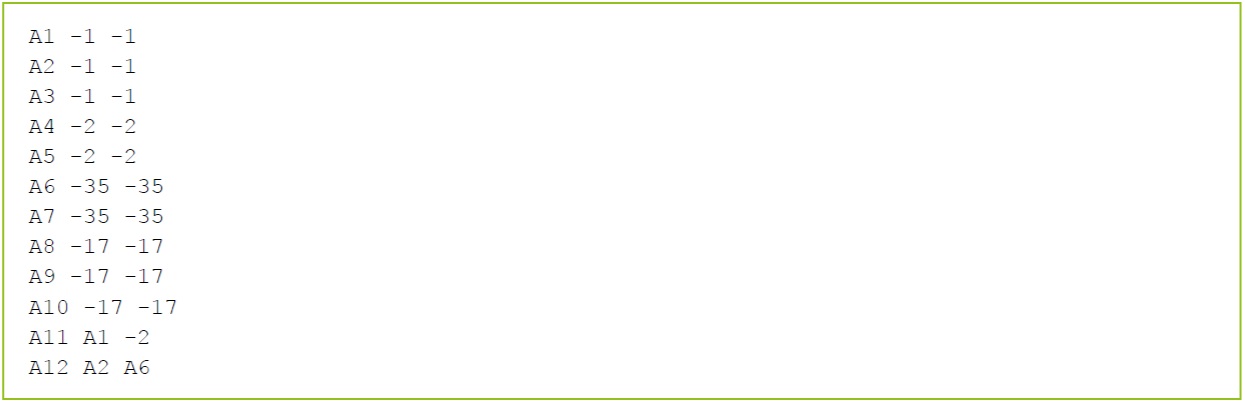
Example. Pedigree file with genetic groups for unknown parents

5.1.5.1. Syntax of multiple large base populations using Westell grouping

PEDFILE <pedigree file> [!GROUPS <value>]
<field animal> <field type>
<field sire> <field type>
<field dam> <field type>

Qualifier:

!Groups <value> The qualifier GROUPS means that genetic groups are included in the pedigree. Genetic groups need to be coded with negative integer values. With <value>, it is possible to specify whether these Genetic group effects should be modelled as fixed (value = 0.0) or as random (value > 0.0). In practice, !GROUPS does not need to be set at a much higher value than about 3.

5.1.5.2. Associated output files for Westell grouping

Output file	Description
Solani.txt	Solutions of the direct genetic effect including the genetic group effects
	when the field type of the ID is integer
Solani.out	Solutions of the direct genetic effect including the genetic group effects
	when the field type of the ID is alphanumerical
Relani.txt	Approximate reliabilities when the field type of the ID is integer
Relani.out	Approximate reliabilities when the field type of the ID is alphanumerical

5.1.5.3. Syntax of multiple large base populations using precalculated genetic group covariates

PEDFILE <pedigree file>
<field animal> <field type>
<field sire> <field type>
<field dam> <field type>
REGFILE
<field animal> <field type I or A>
REG01 <covariate file name REG01> !GGCOV !REGTYPE F/R/H
[REGPARFILE]
[REG01 <parameter file name REG01>]
MODEL
<trait> ~ <fixed effects> !RANDOM REG(1) <other random effects>

Qualifier:

!GGcov
The qualifier !GGcov specifies which external covariate file contains genetic group covariates. If !MakeGGcov is specified, there is no need to specify a file name for the covariate file with !GGcov

REG(...) or hpReg(...)
When using the MiX99 solver, the REG function can be used to fit a genetic group covariate file in the model of a trait. If the genetic group covariate file is fitted for any trait through REG(...), the covariates will be fitted for all traits, even the ones for which REG(...) is not specified.
The numbers in the REG(...) function link to the number in the label of the general covariate file in the REGFILE section (and the REGPARFILE section). The numbers may be specified individually as (1, 2, 3, 4) or as a range, indicated by two subsequent full stops, for example (1..4), or a combination of both. The index is the individual’s ID in the data file.
When using the hpblup solver, the hpReg function can be used to fit a genetic group covariate file in the model of a trait. Note that a genetic group covariate file fitted through hpReg(...) is only fitted for the traits for which it is in the model.
The hpReg function has two parameters. The first one is the label number of the covariate file in the REGFILE section. The second parameter is the field name in the data file of the index of the covariate file.

5.1.5.4. Syntax of multiple large base populations using calculated genetic group covariates

PEDFILE <pedigree file> !MAKEGGCOV
<field animal> <field type>
<field sire> <field type>
<field dam> <field type>
REGFILE
<field animal> <field type I or A>
REG01 !GGCOV !REGTYPE F/R/H
[REGPARFILE]
[REG01 <parameter file name REG01>]
MODEL
<trait> ~ <fixed effects> !RANDOM REG(1) <other random effects>

Qualifier: !MakeGGcov
The qualifier !MakeGGcov is optional and triggers MiXBLUP to set up a covariate matrix Q of the number of genetic groups by the number of individuals in the analysis. The covariates are stored in a standard covariate file.

5.1.5.5. Associated output files for genetic group covariates

Output file	Description
Solani.txt	Solutions of the direct genetic effect when the field type of the ID is integer
SolaniGG.txt	Solutions of the accumulated genetic group effects for each individual
Solanitot.txt	Solutions of the direct genetic effect including the genetic group effects
	when the field type of the ID is integer
GeneticGroupsInQ.txt	Original genetic group label by column in the covariate file
Solani.out	Solutions of the direct genetic effect when the field type of the ID is alphanumerical
Solreg_mat.txt	Solutions of genetic group covariates, along with solutions
	of any other external covariates
SolaniGG.out	Solutions of the accumulated genetic group effects for each individual
Solanitot.out	Solutions of the direct genetic effect including the genetic group effects
	when the field type of the ID is alphanumerical
Relani.txt	Approximate reliabilities when the field type of the ID is integer
Relani.out	Approximate reliabilities when the field type of the ID is alphanumerical

5.1.6. Unknown parents are from multiple related base populations (metafounders)

If individuals without known parents originate from multiple base populations, it may be reasonable to assume that these base populations are not unrelated. Information on average relationships within and between base populations may come from genotyped descendants of the unknown parents or from discarded pedigree information. Related base populations are generally referred to as metafounders. Average genetic relationships within and between metafounders are presented to the solver in an inverse gamma matrix. In case of relationships because of discarded pedigree and/or genotype information, the user needs to calculate the gamma matrix prior to the evaluation and specify the name of the matrix. If the relationships are entirely based on genotypes included in the evaluation, then MiXBLUP can also calculate the gamma matrix. Metafounders are presented in the pedigree file in the same way as genetic groups, i.e. as negative integers. The file with the gamma matrix should be a text file in I-J-Value format, i.e. metafounder ID of row, metafounder ID of column, average genetic relationship. Only non-zero genetic relationships of the lower triangular part of the matrix need to be specified.

5.1.6.1. Syntax of multiple related base populations using metafounders

PEDFILE <pedigree file> !Metafounders
<field animal> <field type>
<field sire> <field type>
<field dam> <field type>

Qualifier:

!Metafounders
or
!Metafounders <file with gamma matrix>
This qualifier indicates that base populations in the pedigree are related. If a file with the gamma matrix is specified, the gamma matrix is coded for either the default or the hpblup solver. If a file with the gamma matrix is not specified, the gamma matrix with genomic relationships within and between metafounders is estimated from available genomic information. Metafounders are fitted using this gamma matrix with coded IDs, and QP transformation.

5.1.6.2. Associated output files for metafounders

Output file	Description
Solani.txt	Solutions of the direct genetic effect when the field type of the ID is integer
Solani.out	Solutions of the direct genetic effect when the field type of the ID is alphanumerical
Relani.txt	(Weighted) inverse genomic relationship matrix
Relani.out	Approximate reliabilities when the field type of the ID is integer
ExtRelMat_tri.txt	Weighted inverse genomic relationship matrix
gamma.dat	gamma matrix with relationships within and across metafounders

5.2. Preparing genomic data

5.2.1. General

Genomic data can be used to estimate true genetic similarity between individuals. Genomic data consists of a large number of bi-allelic SNP markers.

5.2.2. Recommended file formats

5.2.2.1. Genomic data

It is recommended to provide genomic data as genotypes, which is the count of one of the two alleles. This may be provided as a space-separated or dense text file or in binary format.

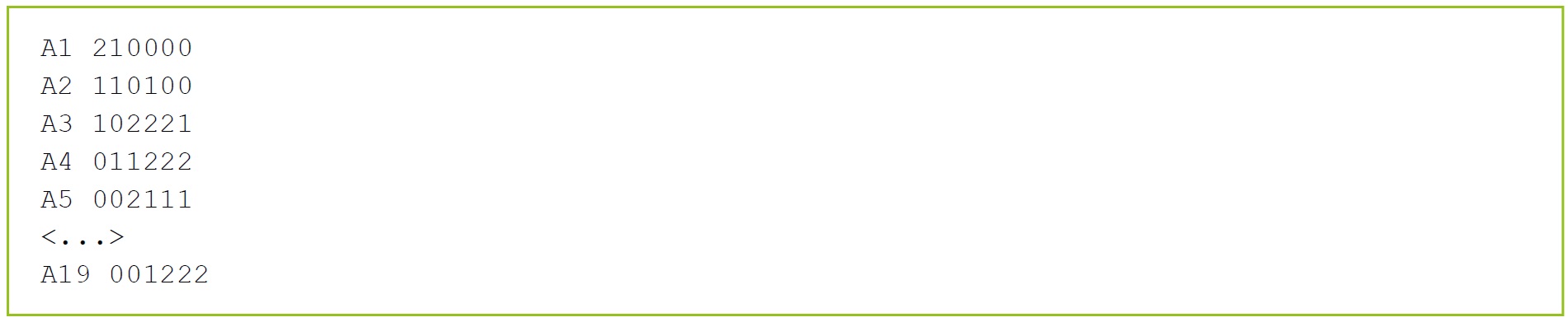
Example. Genotype file with marker genotype data per animal in dense format. It contains the number of copies per locus of the allele with the highest number (11=0, 12=1 and 22=2).

The recommended way to provide genomic data is binary plink format. It consists of three files. The .bim file contains the SNP marker details in text format, the .fam file contains details of genotyped individuals in text format and the .bed file contains the genotype of each individual for each SNP marker in compressed binary format. For GBLUP and single-step GBLUP, genomic data may be also provided as alleles, either using pairs of alleles on a single record per individual or splitting pairs of alleles onto two records per individual. This may be useful for using multi-allele loci. See appendix <Genomic data files> for details.

5.2.2.2. Allele frequencies

If the user does not want to use allele frequencies calculated from the data, then pre-calculated allele frequencies can be supplied as an additional input file, The file specified should contain for each locus the allele frequency of the allele with the highest integer code, if the genetic marker file contains alleles. The file specified should contain for each locus the frequency of the allele of which the homozygote genotypes are coded as 2. The structure of the file is <locus number in order of the genetic marker file> <allele frequency>. Pre-calculated allele frequencies are supported for GBLUP, single-step GBLUP, SNPBLUP and single-step SNPBLUP.

Example. Pre-calculated allele frequency per locus of allele coded with the highest integer code for 6 loci

5.3. Genetic similarity from pedigree only

5.3.1. General

MiXBLUP supports analyses using a pedigree that consists of individuals and their parents (animal model). A sire model with sires and maternal grandsires in the pedigree file is currently not supported in MiXBLUP.

5.3.2. Syntax of using pedigree BLUP

PEDFILE <pedigree file> [!SKIP <n lines>]
<field animal> <field type>
<field sire> <field type>
<field dam> <field type>
[<field block variable> <field type> !BLOCK]

Qualifiers:

!SKIP
The SKIP qualifier may be used to skip the first n lines of the pedigree file. This is useful for ignoring a header.

IF(HPB)

5.4. Genetic similarity from genomic data

5.4.1. Genetic similarity from genomic data with unknown pedigree

5.4.1.1. General

In an evaluation with genomic data only, all individuals are genotyped. Genomic data can be used to calculate a genomic relationship matrix. The inverse of this matrix is used to include genetic similarity between individuals. A range of inverse genomic relationship matrix files can be created by MiXBLUP to be incorporated in the evaluation (chapter 5.4.1.2.). The marker effect solutions can be estimated afterwards (chapter 5.4.4.).

An alternative method to estimate genomic breeding values is to model the direct genetic effect with a random regression on number of copies of a SNP allele for a large number of loci (chapter 5.4.1.3. and chapter 5.4.1.4.). Direct genomic values for genotyped individuals without data can be estimated afterwards from the marker effect solutions.

5.4.1.2. Syntax of using GBLUP

ERMFILE <Name file with genetic markers> !CONSTRUCT Ginv
<animal ID> <field type>
!METHOD <Yang, VanRaden or VanRaden2> (optional; default VanRaden2)
!ALFREQ <file name> (optional; default calculated from data)
!CROSSBRED <number of breeds> <file name> (optional; default single breed)
!INFORMATIVE (optional; default is to use all SNPs)
!DENSE <field number> (optional; default string of markers in free format, field number is column with dense genotypes)
!MAF <minimum allele frequency> (optional; default is 0.005)
!NUMPROC <number of processors to be used by calc_grm> (optional; default is 1)
!SKIP <n lines> (optional; default is reading all lines)
!GFROMDISK (optional; default is to store relationship matrix in memory during solving)

Qualifiers:

!CONSTRUCT Ginv
The !CONSTRUCT qualifier is optional and indicates that the external relationship matrix has not been calculated yet and needs to be calculated in the MiXBLUP parser. For a GBLUP analysis, the argument of !CONSTRUCT is Ginv, for an inverse genomic relationship matrix.

!METHOD <Yang, VanRaden or VanRaden2>
The !METHOD qualifier is optional and specifies whether the method of Yang (Nat Genet 42:565-569) or the method of VanRaden (J Dairy Sci 91: 4414-4423) is used. The VanRaden2 method is the default.

!ALFREQ <file name>
The !ALFREQ qualifier is optional and allows the use of pre-defined allele frequencies per locus from the file specified. By default, the base population allele frequencies are calculated from the data.

!CROSSBRED <number of breeds> <name file with breed composition per animal>
The !CROSSBRED qualifier is optional and can be used for multi-breed analyses that may or may not include crossbred animals. There are two arguments. The one argument is the number of pure breeds in the analysis. The other argument is the name of the file with the breed composition of the animals in the genetic marker file. The !CROSSBRED option will consider relationships between all animals, regardless of their breed composition, using for each animal allele frequencies that are specific for their breed composition.

!INFORMATIVE
The !INFORMATIVE qualifier is used to include only genetic markers with all three genotypes present in the population of genotyped individuals. The default is to include all genetic markers with more than just one allele in the data.

!DENSE [<field number of dense column>]
The !DENSE qualifier must be specified if the genetic marker data is presented as a sequence of genetic markers without spaces. If the dense column is not the second field in the record, the field number of the dense column needs to be specified after the qualifier, for example !DENSE 4. If !DENSE is not specified for a file with dense genetic marker data, MiXBLUP will give a column-width error, as it attempts to read the dense genetic markers as a single column. By default, MiXBLUP expects space-separated genetic markers.

!MAF
The qualifier !MAF is optional and is used to set the minimum allele frequency of genetic markers to be included in the analysis. The default value is 0.005. Use !MAF 0.0 to include all SNP with more than one allele in the data.

!NUMPROC
The !NUMPROC qualifier can be used to specify the number of threads to be used by calc_grm.

!GFROMDISK
The !GFROMDISK qualifier instructs the solver to read the inverse genomic relationship matrix from disk during solving. This was the only option in previous versions of MiXBLUP. The default is to keep this matrix in memory, which is more demanding for memory requirement, but it saves the time to read this matrix every iteration. It is specified in the SOLVING section of the MiXBLUP instruction file.

5.4.1.3. Syntax of using SNPBLUP for the MiX99 solver

SNPFILE [!CENTER] [!NOIMPUTE] [!MISSCOMB 0.01] [!MISSPERLOC 0.01] [!NOPRUNE] [!CALCSNPVAR] [!MINGENFREQ] [!GBSORTSNP ] [!SAMEORDER]
<field animal> <field type I or A>
SNP01 <file name SNP01> !REGTYPE R [!IDCOL <n>] [!STARTCOV <n>] [!LASTCOV <n>]
SNP02 <file name SNP02> !REGTYPE R [!IDCOL <n>] [!STARTCOV <n>] [!LASTCOV <n>]
<...>
SNP99 <file name SNP99> !REGTYPE R [!IDCOL <n>] [!STARTCOV <n>] [!LASTCOV <n>]
[SNPPARFILE (required only for !REGTYPE H or for !REGTYPE R if !CALCSNPVAR is not specified)
SNP01 <file name SNP01>
SNP02 <file name SNP02>
<...>
SNP99 <file name SNP99>]
MODEL
<trait> ~ <fixed> !RANDOM SNP(1,2,8..15,23) # so no need for G(...) in the model

Sections:

SNPFILE
The SNPFILE section specifies the name of one or more SNP covariate files and its attributes, such as column numbers, dense or space-separated SNPs and whether one variance for all SNPs is used or an individual variance for each SNP. The section also has a number of qualifiers that apply to all SNP covariate files.

SNPPARFILE
The SNPPARFILE section specifies the name of a parameter file for each SNP covariate file for which the SNP covariates are fitted as a random regression (so !REGTYPE is either ‘r’ or ‘h’). The SNPPARFILE section does not have any associated qualifiers. The lines of the SNPPARFILE section each contain two columns. The first column is the label that links the parameter file to the SNP covariate file. The second column is the name of the file.

Qualifiers:

The file-independent qualifiers of SNPFILE are typically specified on the first line of the SNPFILE section. These are:
!CENTER
The !CENTER qualifier is optional and scales all SNP’s to a mean of 0 and standard deviation of 1. For details, see Stranden and Christensen (2011). Centring the SNPs affects the fixed effect solutions, but not the SNP effect solutions. Centering may enhance convergence of the PCG iteration.

!MISSCOMB <maximum fraction of SNPs missing>
The MISSCOMB qualifier is optional and can be used to specify the tolerance level of missing combinations of animal and SNP. Above the tolerance level, a warning is printed that the analysis may not yield meaningful results, but the analysis continues. If !MISSCOMB is not specified, the tolerance level is 0.001 of all combinations of animal and SNP marker.

!MISSPERLOC <maximum fraction of SNPs missing per locus>
The MISSPERLOC qualifier is optional. It specifies the tolerance level of missing SNPs per locus. Loci with too many missing SNPs are written to CheckDataSNP.log and a warning is printed. If !MISSPERLOC is not specified, the tolerance level is 0.05 of all genotypes for the locus (call rate of 95%).

!NOIMPUTE
The !NOIMPUTE qualifier can be used to avoid automatic imputation of missing SNPs with the average SNP value of the locus. If !NOIMPUTE is specified, then animals with one or more missing SNPs get a genomic breeding value of -99999 in the solanigen.txt file. If !NOIMPUTE is not specified, then the average SNP value of the locus is used in the calculation of the genomic breeding value.

!NOCHECK
The !NOCHECK qualifier can be used omit any imputing, pruning, centring or checks of SNP covariates, which must be on the scale 0 to 2.

!NOPRUNE
The !NOPRUNE qualifier can be used omit the verification that all SNPs are informative and the exclusion of non- or less-informative SNPs.

!MINGENFREQ
The !MINGENFREQ qualifier is optional and can be used to vary the definition of a less-informative SNP. If the frequency of the minor SNP genotype is below the threshold, it is considered to be less-informative and it will be excluded from the analysis, unless !NOPRUNE has been specified. The default threshold is 0, which does not remove any SNP markers.

!CALCSNPVAR
The optional !CALCSNPVAR qualifier can be used to calculate the SNP variance from the direct genetic variance in the parameter file specified in the PARFILE section. The CALCSNPVAR qualifier must not be specified if one or more SNP files have SNP-specific variances (!REGTYPE H). If one or more SNP files are fixed (!REGTYPE F), the SNP variance is calculated using the remaining SNP files with !REGTYPE R. When !CALCSNPVAR is specified, the SNPPARFILE section is ignored.

!GBSORTSNP <amount of memory in Gb>
The qualifier !GbSortSNP only applies to the MiX99 solver. It is optional and can be used to control the use of memory for sorting SNP covariate records in the order of the data file. SNP covariate records are sorted in blocks of records. !GBSORTSNP determines the size of such a block of records to be sorted simultaneously. The default allocation is 16 Gb. The number of blocks of records is the number of times a SNP covariate file has to be read, so a small memory allocation increase the time needed to sort the SNP covariates.

!SAMEORDER
The qualifier !SameOrder only applies to the MiX99 solver. If there are multiple SNP covariate files and records in each file are in the same order of individual ID, then !SAMEORDER can be used. MiXBLUP will sort all SNP covariate files simultaneously. Note that memory allocated with !GBSORTSNP is now used for multiple SNP covariate files instead of a single file.

The second line of the SNPFILE section specifies the animal ID code that can be used to link the data and the SNP covariate files.
The following lines each specify a SNP covariate file. Each line starts with a label. The label links the SNP covariate file to the corresponding SNP parameter file. The label must have the form ‘SNPxx’ where xx is a number between 01 and 99. The second field contains the name of the SNP covariate file. The additional fields contain one or more file-specific qualifiers. These are:

!REGTYPE
The file-specification line must contain the !REGTYPE qualifier. It specifies how the covariates in the file are fitted in the model. If ‘f’ is specified, the covariates in the file are fitted as a fixed regression. Covariates fitted as a fixed effect do not have a variance associated with it, so it is not necessary to specify a parameter file in the SNPPARFILE section. If it is present, it is ignored. If ‘r’ is specified, the covariates in the file are fitted as a random regression with a single variance for all covariates in the file. The variance is specified in the corresponding parameter file in the SNPPARFILE section. If ‘h’ is specified, the covariates in the file are fitted as a random regression, each with their own variance. The covariate-specific variances are specified in the corresponding parameter file in the SNPPARFILE section.

!IDCOL
The !IDCOL qualifier is optional and specifies which field in the SNP covariate file contains the ID of the genotyped animal. If it is omitted, it is assumed that the ID is in the first field of the record (so the default is !IDCOL 1).

!STARTCOV
The !STARTCOV qualifier is optional and specifies which field contains the first SNP covariate. If it is omitted, it is assumed that the SNP covariates start in the second field of the record (so !STARTCOV 2).

!LASTCOV
The !LASTCOV qualifier only applies to the MiX99 solver. It is optional and specifies which field contains the last SNP covariate of the file to include in the model. If it is omitted, it is assumed that all fields after the first SNP covariate contain SNP covariates to include in the model.

SNP(...)
The SNP function only applies to the MiX99 solver. It can be used in the MODEL section to specify which SNP covariate files should be fitted in the model of a trait. If a SNP covariate file is specified, then all specified SNP covariates in the file will be fitted. The number in the SNP(...) function links to the number in the label of the SNP covariate file. The numbers may be specified individually as (1, 2, 3, 4) or as a range, indicated by two subsequent full stops, for example (1..4), or a combination of both. When SNP(...) is specified, it is not necessary to specify the G(...) function to specify a genetic effect, but it is possible, for example to specify a maternal genetic effect. Despite what the use of SNP(...) in the MODEL section may suggest, all SNP covariate files used in any trait are fitted for all traits.

5.4.1.4. Syntax of using SNPBLUP for hpblup solver

SNPFILE [!CENTER] [!NOIMPUTE] [!MISSCOMB 0.01] [!MISSPERLOC 0.01 [!NOPRUNE] [!CALCSNPVAR] [!MINGENFREQ]
<field animal> <field type I or A>
SNP02 <file name SNP02> !REGTYPE R [!IDCOL 1] [!STARTCOV 2] [!PLINK]
[SNPPARFILE (required only for !REGTYPE H or for !REGTYPE R if !CALCSNPVAR is not specified)
SNP02 ]
MODEL
<trait> ~ <fixed> !RANDOM hpSNP(2,<field animal>) [hpSNP(2,<field dam>)]

Qualifiers:

Please note: the qualifiers !GbSortSNP, !SameOrder and !LastCov have no effect when using the hpblup solver.

hpSNP(<label number>,<index field>)
The hpSNP function is used to specify which SNP covariate files should be fitted in the model of a trait. Unlike for the MiX99 solver, the SNP covariate file is not fitted automatically for all traits. The first parameter of the hpSNP function is the number in the label of the SNP covariate file. The second parameter is the index field in the data file. Every combination of label and index field requires a separate hpSNP function in the model of a trait.

5.4.2. Genetic similarity from pedigree and genomic data

5.4.2.1. General

If pedigree data is available or if some individuals are not genotyped, a single-step genomic BLUP model can be used. There are three approaches. In the first approach, an inverse genomic relationship matrix is used (ssGBLUP), either explicitly or implicitly in decomposed form. The inverse genomic and pedigree relation matrices are blended. There are various ways to do this (Appendix 3). If the number of genotyped individuals is below 40,000, it is recommended to use the full inverse of weighted G (chapter 5.4.2.2.. If the number of genotyped individuals is higher, it is recommended to use the component-wise Ta decomposition of G (ssGTacBLUP; chapter 5.4.2.3.. The second approach is mathematically equivalent to ssGBLUP and fits every SNP marker as a covariate. The method implemented was developed by Liu et al. (2014) and contains SNP covariates and a residual polygenic effect. A genomic estimated breeding value (GEBV) is calculated for all individuals, which is the sum of the direct genomic value, calculated from the SNP effects, and the residual polygenic breeding value. This method is called single-step SNP BLUP (ssSNPBLUP; chapter 5.4.2.4.). If the number of animals with both a phenotype and a genotype is sufficiently large for all traits, then SNP effect estimates are quite stable for a number of subsequent evaluations. The third approach uses previously estimated SNP effects to calculate direct genomic values (DGV) for genotyped animals. These DGV are fitted as prior information in a pedigree BLUP evaluation (DGV-PBLUP; chapter 5.4.2.5. and 5.4.2.6.). DGV-PBLUP can be used with ssGTacBLUP and ssSNPBLUP. A full genomic evaluation is needed periodically to re-estimate SNP effects. DGV-PBLUP provides a substantial reduction in runtime and computing resources. The number of subsequent evaluations for which DGV-PBLUP can be used, depends on multiple factors, such as the size of the phenotype and genotype datasets. DGV-PBLUP is only available for the hpblup solver.

5.4.2.2. Syntax of SSGBLUP: single-step genomic BLUP with full inverse of a weighted G

ERMFILE <Name file with genetic markers> !CONSTRUCT SSmat
<animal ID> <field type> !LAMBDA <weighting factor G matrix, 0.0-1.0> (optional; default 1.0)
!ALPHA <weighting factor, 0.0-1.0> (optional; default is 0.95)
!BETA <weighting factor, 0.0-1.0> (optional; default is 1.0-ALPHA)
!OMEGA <weighting factor, 0.0-1.0> (optional; default is LAMBDA)
!SINGLESTEP
[INBRFILE <inbreeding coefficient file> !IDCOL <number> !INBRCOL\ <number>]
PEDFILE <pedigree file> [!CALCINBR]
<individual ID> <field type>
<sire ID> <field type>
<dam ID> <field type>

Any qualifier of ERMFILE described in chapter 5.4.1.1. can also be used for a weighted inverse genomic relationship matrix. Specific qualifiers:

!CONSTRUCT SSmat
The !CONSTRUCT qualifier indicates that the external relationship matrix has not been calculated yet and needs to be calculated in the MiXBLUP parser. For a ssGBLUP analysis with a weighted inverse genomic relationship matrix, the argument of !CONSTRUCT is SSmat.

!LAMBDA
!ALPHA
!BETA
!OMEGA
The !LAMBDA, !ALPHA, !BETA and !OMEGA qualifiers are the fudge parameters suggested by Misztal and coworkers. They are optional and can be used to give more weight to numerator relationship matrix (A-1) in the construction of the blended matrix (H-1):

By default, lambda is set to 1, omega to lambda, alpha to 0.95 and beta to 0.05.

!SINGLESTEP
The qualifier !SINGLESTEP is used to indicate that the MiXBLUP kernel should calculate elements of the H-inverse from a G-inverse, the pedigree file and a file with inbreeding coefficients. This option requires a matrix that is set up using !CONSTRUCT with argument SSmat.

5.4.2.3. Syntax of ssGTacBLUP: single-step GBLUP with component-wise Ta decomposition of a weighted G

ERMFILE <Name file with genetic markers> !CONSTRUCT ssMat !Tac !SingleStep
<animal ID> <field type>

Any qualifier of ERMFILE described in chapter 5.4.1.2. and chapter 5.4.2.2. can also be used for a decomposition of a weighted inverse genomic relationship matrix. Specific qualifiers:

!CONSTRUCT SSmat
The !CONSTRUCT qualifier indicates that the external relationship matrix has not been calculated yet and needs to be calculated in the parser.

!Tac
For a ssGBLUP analysis with a decomposition of a weighted inverse genomic relationship matrix, add the qualifier !Tac. Component-wise Ta decomposition of a weighted G is only more efficient if the number of genotyped individuals is substantially larger than the number of SNP markers. If the number of genotyped individuals is between 40,000 and say 1.5 times the number of SNP markers, then ordinary Ta decomposition using the qualifier !Ta instead of !Tac may be more efficient.

5.4.2.4. Syntax of ssSNPBLUP: single-step BLUP using SNP genotypes as covariates

PEDFILE <file name pedigree file> !CalcInbr !Beta <value>
<field individual ID> <field type I or A>
<field sire ID> <field type I or A>
<field dam ID> <field type I or A>
<...>
SNPFILE [!CalcSNPvar] !NoCheck !NoPrune
<field individual ID> <field type I or A>
SNP01 <file name SNP01> !REGTYPE R [!IDCOL <value>] [!STARTCOV <value>]
<...>
MODEL
<trait> ~ <...> !RANDOM hpSNP(1,<individual ID field>) [hpSNP(1,<dam ID field>)] G(<field individual ID>[,<dam ID field>])

Qualifiers:

!Beta
The qualifier !Beta is optional and can be used to specify the fraction of residual polygenic variation. It must not be zero and should be at least 0.05, which is the default value if !Beta is not specified. The qualifier !Beta can be specified in the PEDFILE or the SOLVING section for ssSNPBLUP. The qualifier !Alpha cannot be specified for ssSNPBLUP but is calculated as 1 – Beta.

!CalcSNPvar
The optional !CALCSNPVAR qualifier can be used to calculate the SNP variance from the direct genetic variance in the parameter file specified in the PARFILE section. The CALCSNPVAR qualifier must not be specified if one or more SNP files have SNP-specific variances (!REGTYPE H). If one or more SNP files are fixed (!REGTYPE F), the SNP variance is calculated using the remaining SNP files with !REGTYPE R. When !CALCSNPVAR is specified, the SNPPARFILE section is ignored.

!NoCheck, !NoPrune
It is advised to use !NoCheck and !NoPrune if GEBV of young individuals with genotype, but not phenotype or progeny, are calculated in a separate analysis. Not using these options may lead to non-compatible SNP covariate files of the main evaluation and the evaluation of young genotyped individuals, which will result in an error.

5.4.2.5. Syntax of DGV-Pedigree BLUP from Tac: using previously estimated SNP effects as prior information in pedigree BLUP

PEDFILE <file name pedigree file> !CalcInbr
<field individual ID> <field type I or A>
<field sire ID> <field type I or A>
<field dam ID> <field type I or A>
<...>
ERMFILE <genotype file in plink format> !Plink !CONSTRUCT ssMat !SingleStep [!Tac or !Ta] <field individual ID> <field type I or A>
!METHOD VanRaden
!MAF 0.000
!ALPHA 0.95
!DGVPBLUP <name file with SNP effect solutions from Tac/Ta evaluation>
!AlFreq <name file with estimated allele frequencies from Tac/Ta evaluation>
MODEL
<trait> ~ <...> !RANDOM G(<field individual ID>[,<dam ID field>])
SOLVING
!hpblup

Qualifiers:

!DGVPBLUP
The qualifier !DGVPBLUP can be used to specify that old solutions for SNP effects should be used as prior information. For a component-wise Ta decomposition, SNP effect estimates are written to a file called snpeffects_ta.dat. The specified file should be a copy of this file.

!AlFreq
The qualifier !AlFreq is mandatory if !DGVPBLUP is used. The file specified should come from the same evaluation as the SNP effect estimates. Allele frequencies are written to calculated_all_freq.dat. The specified file should be a copy of this file.

!MAF 0.000
It is advised to use a minor allele frequency of 0.0%. Not using this option may lead to non-compatible SNP and allele frequency files, which will result in an error.

5.4.2.6. Syntax of DGV-Pedigree BLUP from ssSNPBLUP: using previously estimated SNP effects as prior information in pedigree BLUP

PEDFILE <file name pedigree file> !CalcInbr !Beta <value>
<field individual ID> <field type I or A>
<field sire ID> <field type I or A>
<field dam ID> <field type I or A>
<...>
SNPFILE [!CalcSNPvar] !NoCheck !NoPrune !DGVPBLUP <name file with SNP effects solutions> !AlFreq <name file with estimated allele frequencies>
<field individual ID> <field type I or A>
SNP01 <file name SNP01> !REGTYPE R [!IDCOL <value>] [!STARTCOV <value>]
<...>
MODEL
<trait> ~ <...> !RANDOM hpSNP(1,<individual ID field>) [hpSNP(1,<dam ID field>)] G(<field individual ID>[,<dam ID field>])

Qualifiers:

!DGVPBLUP <name of file with estimated SNP effects>
The qualifier !DGVPBLUP can be used to specify that old solutions for SNP effects should be used as prior information. For a single-step SNPBLUP evaluation, SNP effect estimates are written to solutions_mixblup.dat. The file Solreg_mat.txt can also be used and is considerably smaller. The specified file should be a copy of one of these file.

!AlFreq
The qualifier !AlFreq is mandatory if !DGVPBLUP is used. The file specified should come from the same evaluation as the SNP effect estimates. Allele frequencies are written to calculated_all_freq.dat. The specified file should be a copy of this file.

!MAF 0.000 !NoCheck !NoPrune
It is advised to use a minor allele frequency of 0.0%, and the !NoCheck and !NoPrune options. Not using these options may lead to non-compatible SNP and allele frequency files, which will result in an error.

5.4.3. Modelling a genetic difference between genotyped and non-genotyped individuals with the hpblup solver

5.4.3.1. General

The group of genotyped individuals without genotyped ancestors may not be representative for the base population in the evaluation, which is the group of individuals without known parents. As a result, genomic estimated breeding values are biased in the presence of selection and/or selective genotyping (Vitezica et al., 2011). When genomic relationships were shifted by a constant in their study, the single-step method was unbiased and the most accurate of the methods compared. For ssGBLUP using either a full or APY inverse of G, this constant is automatically applied by calc_grm, unless the !NoScale and !NoReg options are used. For ssGTacBLUP and ssSNPBLUP, this constant can be modelled with a so-called J factor that quantifies for any individual the pedigree relationship with genotyped individuals. For genotyped individuals, the J factor is set to -1. For base animals, the J factor is initialised at 0. For ancestors of genotyped individuals, the J factor (Jn) is estimated using Ann Jn = -Ang Jg, where Ang and Ann are partitions of A-inverse of non-genotyped ancestors by genotyped individuals and non-genotyped ancestors by non-genotyped ancestors, respectively, and Jg, as J factor for genotyped individuals, is a vector containing -1 for all. For all remaining individuals, the J factor is the average of the J factor of the parents. It is possible to do this calculation in the parser. The regression coefficient of each trait on the J factor is estimated on all available records. The impact of a priori assuming that estimates originate from a normal distribution with a given variance (i.e. fitting it as a random effect) is very limited. It is therefore recommended to fit J-factor covariate as a fixed effect. The individual correction for bias, calculated for each trait as regression coefficient times J-factor covariate, is added to the GEBV of the trait for each animal. Note that the J factor will change for non-genotyped individuals if new genotyped individuals are added to an evaluation. The calculation of J-factor covariates requires the genotype file and the pedigree file. An existing J-factor covariate file needs to contain all animals in the pedigree.

5.4.3.2. Syntax of fitting J factor covariate

PEDFILE <file name pedigree file> !CalcInbr !Beta <value> !MakeJcov
<field individual ID> <field type I or A>
<field sire ID> <field type I or A>
<field dam ID> <field type I or A>
<...> REGFILE
<field individual ID> <field type I or A>
REG01 !REGTYPE F !Jcov
<...>
MODEL
<trait> ~ <...> hpReg(1, <field individual ID>) !RANDOM <...>

Qualifiers:

!MakeJcov
The qualifier !MakeJcov is optional and is used to specify the calculation of J-factor covariates.

!Jcov
The qualifier !Jcov marks the covariate file that contains the J-factor covariates. If !MakeJcov is specified, it is not necessary to specify a file name.

hpReg(<number in label of covariate file>, <field individual ID>)
The hpReg function is used to fit the J-factor covariate file in the model of each trait. It is recommended that it be fitted as a fixed effect, by specifying the RegType F qualifier in the REGFILE section and by specifying the hpReg function before the !Random qualifier on each line in the MODEL section.

5.4.4. Obtaining solutions for genetic marker effects with the hpblup solver

Genetic marker effect solutions are provided with the recommended methods of a genomic evaluation, ssGTaBLUP, ssGTacBLUP and ssSNPBLUP. Solutions are present in the file Solreg_mat.txt, which contains just the centred genetic marker effect solutions. The order of fields in Solreg_mat.txt is Trait - Matrix - Covariate - EffectID - Solution - Matrix name. Other supported methods of a genomic evaluation (Appendix XX) require back-solving to obtain genetic marker effect solutions. Back-solving needs to be specified at the start of a genomic evaluation. It cannot be done retrospectively. The option !BackSolve in the SOLVING section can be used for this purpose. Back-solving only yields approximate genetic marker effect solutions, so ssGTacBLUP and ssSNPBLUP are the two recommended methods to obtain genetic marker effect solutions.

5.5. External genetic relationship matrix

5.5.1. General

A range of inverse genetic relationship matrix files can be created by MiXBLUP explicitly or are implicitly incorporated in the analysis. It is also possible to use a previously created inverse genetic relationship matrix or one that as yet cannot be created by MiXBLUP itself. It is not possible to calculate reliabilities with MiXBLUP when using a full external relationship matrix.

5.5.2. Recommended file format

An external relationship matrix must contain the original ID of each individual. This can be a decoded matrix from a previous evaluation or one from an external source. The recommended file format for a dense inverse relationship matrix (most matrix elements are non-zero) is the dense or lower-triangular matrix format. The first line of the dense format contains the number of genotyped individuals and the number of individuals in the core in case of an APY-inverse or 0 otherwise. The second line contains the original ID of each individual separated by one or more spaces. The next lines contain all elements of the lower-triangular part of the matrix up to and including the diagonal element. An external dense relationship matrix may also be provided in stream binary format, recognized from the .stream filename extension. The recommended file format for a sparse inverse relationship matrix is the sparse or I-J-value matrix format. Each line consists at least of three fields: original individual ID of row, original individual ID of column, matrix element. Any other fields on the line are ignored.

5.5.3. Syntax of using an external relationship matrix

ERMFILE <external relationship matrix file> [!SKIP <n lines>] [!ASIS] [!NOORIG] <field individual ID> <field type>

Qualifier:

!SKIP <n lines>
The optional !SKIP qualifier may be used to skip the first n lines of the external relationship matrix file. This is useful for ignoring a header line.

!ASIS
The !AsIs qualifier is optional. It is used to write the external inverse relationship matrix to the kernel without any checks or sorting. This can be specified if the external relationship matrix file is known to be correct, for example because it was created or checked by MiXBLUP in a previous run. The !AsIs qualifier can only be used if the field type of the individual ID is integer. It is ignored when individual ID has alphanumerical field type.

!NOORIG
If the MiX99 solver is used, MiXBLUP converts the coded external inverse relationship matrix file back to the original individual IDs. If this file is not needed for additional analyses, the !NoOrig qualifier can be specified. Especially for very large analyses, the size of this file can be substantial.

Table. Decoded weighted genomic relationship matrices from MiXBLUP evaluations

Solver	Dense matrix format	Sparse matrix format
MiX99 solver - integer ID	ExtRelMat_tri.txt	ExtRelMat.txt
MiX99 solver - alphanumerical ID	ExtRelMatAlphaTri.stream	ExtRelMatAlpha.stream
hpblup solver	Not decoded	Not decoded

5.6. Genetic similarity in case of multiple breeds or lines and crosses

5.6.1. General

There are several ways to correctly model that a genetic evaluation consists of multiple breeds, lines or crosses (referred to as genetic lines in this chapter). The effect of multiple genetic lines can be fitted as a fixed effect in the model, it can be fitted as a separate base population for each genetic line in the pedigree or allele frequencies specific for the genetic lines may be provided.

5.6.2. Fixed effect in the model

In case of the evaluation only containing purebred individuals, the genetic line of the individual may be fitted as a fixed class effect. In case of unstructured crossbreeding, it is recommended to fit a covariate for each genetic line with the percentage of genes for that line, except for one genetic line: a covariate of the most prevalent genetic line should not be fitted in order to avoid singularity of the coefficient matrix. Its effect is then included in the overall mean. In case of purebred breeding and structured crossbreeding, either fixed class effects can be used, or fixed genetic line covariates. See Chapter 7. for the syntax of fitting fixed class effects or fixed covariates. Note that fixed effect estimates of genetic line are not automatically included in genetic effect solutions.

5.6.3. Base population for each genetic line

An alternative way of fitting effects of genetic line is to assign individuals in the base generation to a base population (i.e. genetic group) that is specific for a genetic line. See Chapter 5.1.5. for the syntax of fitting multiple base populations. Solutions of base populations are automatically added to genetic effect solutions.

5.6.4. Allele frequencies specific for a genetic line

A breed composition file can be used to indicate that allele frequencies should be estimated for each line in the breed composition file separately. The breed composition file contains the original animal ID in the first column and contains a number of additional columns that is equal to the number of genetic lines specified. The breed composition may be presented as a number, for example 4 (out of 8 or any other number), as a percentage, for example 50, or as a fraction, for example 0.50. MiXBLUP converts the breed composition of an animal to the value of one breed over the sum of values across breeds. For example in an analysis with four breeds, animal X having 4 0 2 2 as the breed composition will be converted to X 0.500 0.000 0.250 0.250. It is therefore essential that the breed information is complete, so add a column for ‘unknown or other’, if necessary. All columns must be separated by at least one space.

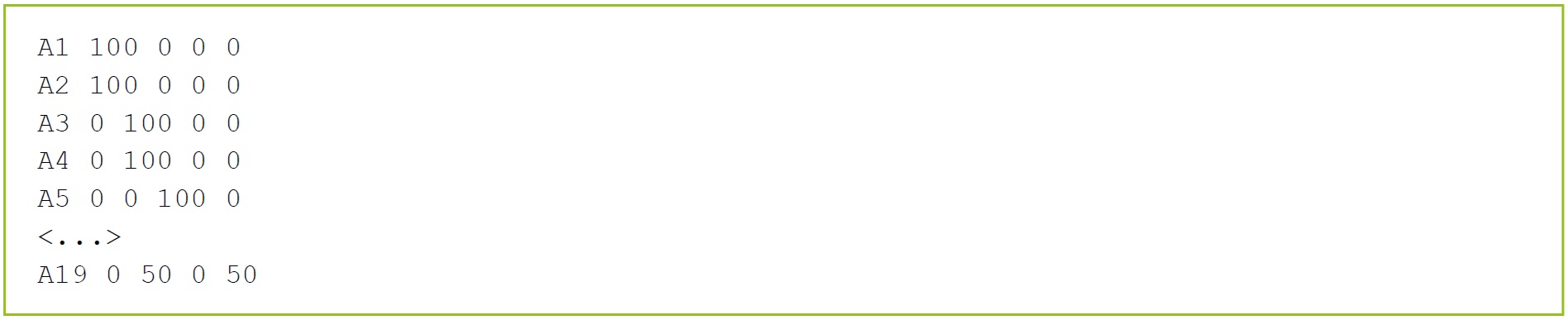
Example. Breed composition file with the percentage of four breeds per animal

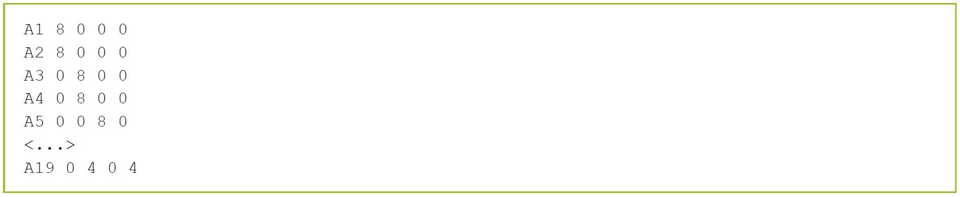
Example. Breed composition file in parts of one eighth of four breeds per animal

5.7. Non-additive genetic similarity

Multiple genetic or genomic relationship matrices will be supported shortly. This includes a genomic dominance or epistasis relationship matrix. This section is pending the release of this feature.

5.7.1. General

Systematic change of populations through genetic selection focuses on additive genetic effects. In reality, there may be interactions between alleles within a locus (dominance), interactions between loci (epistasis), and expression that depends on environmental conditions. Loss of heterozygosity because of inbreeding causes loss of dominance effects and leads to inbreeding depression. Recovering from inbreeding depression after crossbreeding is referred to as heterosis. Breaking up of favorable epistatic effects after repeated crossbreeding is referred to as recombination.

5.7.2. Expected heterosis and recombination in crossbreds

In case of unstructured crossbreeding, it is meaningful to correct for expected heterosis and recombination if genotype information is not available for a large part of the population. Both are a function of the breed fractions of the parents.

Expected heterosis (Het) for genetic line A and B of a crossbred individual is calculated as:

Het~A,B~ = p~sire,A~*p~dam,B~ + p~dam,A~*p~sire,B~

Expected recombination (Rec) for genetic line A and B of a crossbred individual is calculated as:

Rec~A,B~ = p~sire,A~*p~sire,B~ + p~dam,A~*p~dam,B~

Here, p~sire,A~ and p~dam,A~ are the breed fractions of genetic line A for the sire and the dam of the individual. An expected heterosis and an expected recombination term should be fitted for each combination of genetic lines present in the evaluation. Expected heterosis and recombination can be fitted as fixed covariates for each individual in the genetic evaluation. See Chapter 7. for the syntax of fitting a fixed covariate.

5.7.3. Genomic dominance effects (to complete)

5.7.3.1. General

Dominance effects can be estimated from heterozygous loci if all individuals in the evaluation are genotyped. Heterozygosity can be used to calculate an inverse dominance relationship matrix or create a covariate. Genomic dominance can be fitted as an additional random genetic correlated effect.

5.7.3.2. Syntax

ERMFILE <genotype file>
<ID field> I/A
!ConstructDom
CORRFILE
RCE01 !GenRCE !Dominance # no file needed
<...>
SOLVING
!BackSolveDom

Qualifiers:

!Dominance The !Dominance qualifier is used to specify that a random effect with correlated levels

!ConstructDom <...>

!BackSolveDom <...>

5.7.3.3. Output files

Output file	Description

5.7.4. Genomic epistasis effects (to complete)

5.7.4.1. General

Modelling epistasis aims to estimate how pairs or groups of markers interact to affect a phenotype, such as in additive by additive or dominance by dominance interactions. The epistasis relationship matrix is usually constructed using the element-wise product of the (non-inverted) additive or dominance relationship matrices. The inverse of the epistasis relationship matrix is used in the genetic evaluation. Genomic epistasis is fitted as an additional random correlated genetic effect.

5.7.4.2. Syntax

ERMFILE <genotype file>
<ID field> I/A
!ConstructEpist
CORRFILE
RCE01 !GenRCE !Epistasis # no file needed <...> SOLVING

Qualifiers:

!Epistasis
<...>

!ConstructEpist
<...>

5.7.4.3. Output files

Output file	Description

5.8. Genetic similarity in case of polyploidy or mixed ploidy

5.8.1. General

The MiXBLUP software was designed originally to support breeding value estimation for diploid species. Although rare in mammals, a mix of diploid and polyploid individuals can be found in species like salamander, frog, trout, salmon, and various insect species. Support for mixed ploidy is currently only available for expected genetic similarity from pedigree. The underlying assumption is that founder animals in the pedigree are from a single large population. Unknown parent groups are currently not supported for polyploidy or mixed ploidy.

5.8.2. Required format of pedigree file

A pedigree file in which some or all individuals are non-diploid, contains at least seven fields. The first seven fields are defined as described in the table below.

Table. Description of fields in a pedigree record for a mixed ploidy pedigree

Field in pedigree record	Description
1	Individual ID
2	Sire ID
3	Dam ID
4	Ploidy level of the gamete transmitted by the sire
5	Ploidy level of the gamete transmitted by the dam
6	Probability that two gametic genes, drawn at random from a randomly selected locus, are inherited from a single parental chromosome (sire)
7	Probability that two gametic genes, drawn at random from a randomly selected locus, are inherited from a single parental chromosome (dam)

Ploidy level of the gamete of a parent of a diploid individual is 1. In that case, the probability that two gametic genes, drawn at random from a randomly selected locus, are inherited from a single parental chromosome is 0. For polyploid individuals, the latter probability is 0 if there is no identity by descent within a gamete, it is 1 if the polyploid gamete was transmitted by a double-haploid individual, and it is between 0 and 1 if there is recombination.

5.8.3. Syntax

PEDFILE pedigree_ploidy.txt !polyploid !CalcInbr
<field individual ID> <field type I or A>
<field sire ID> <field type I or A>
<field dam ID> <field type I or A>
ploidy_sire I
ploidy_dam I
prob_sire I
prob_dam I

Qualifier:

!Polyploid
The !Polyploid qualifier is used to specify that the pedigree contains non-diploid individuals. In that case, MiXBLUP expects each pedigree record to consist of at least seven fields instead of three fields. Without !Polyploid, the four additional fields in the pedigree are ignored. The use of !Polyploid results in an (implicit) inverse pedigree relationship matrix that takes ploidy level of individuals into account. An inverse genomic relationship matrix that takes differences in ploidy into account is currently not supported.

6. Components of variance and covariance among traits

Components of variance and covariance among traits are normally specified in the general parameter file. Additional covariance components for covariates in a covariate file need to be specified in separately labelled parameter files. Heterogeneous residual variances also need to be specified in a separate file. This chapter describes how to specify components of variance and covariance among traits.

6.1. General parameter file

6.1.1. General

The trait (co)variance components file contains the between-trait variance-covariance matrices of any random effects in the statistical model. There are two options for the format of the general parameter file: (1) in lower-triangular-matrix form and (2) in sparse-matrix form. It is strongly recommended to use the lower-triangular-matrix format. The instruction file specifies the name of the trait (co)variance components file. The trait (co) variance components file is located by default in the work directory, but can be in another folder if specified in the name of the file.

6.1.2. Input file in lower-triangular-matrix format

The lower-triangular-matrix form is the default option and strongly recommended. In this form, the trait covariance components file can be specified as a lower-triangular matrix using trait names to identify the components. This is the most user-friendly way. The name of the random effect is given at the top of the matrix and the names of the traits are given at the start of each line of the matrix.

• The lower triangular matrices and the traits within a matrix can be specified in any order. It means that the order given in the MODEL section of the instruction file is not leading.
• The number of traits in the matrices can be larger than the number of traits specified in the model section. Only the lines for which the name has been specified in the model section will be used.
• The order of the column names must be the same as the order of row names, so variance components are on the diagonal.
• Restriction: in case of a marker-assisted BLUP model with the use of haplotype variance-covariance matrices, each matrix needs to be named and numbered, e.g. GIV1, GIV2, etc. The name GIV refers to the use of the General Inverse Variance (GIV) function in the model. The order of matrices must be the same as the order of haplotypes given in the model lines of the instruction file. See Example 5.4 in the Appendix.
• For all direct and indirect genetic effects (e.g. animal, dam, mate), it should be specified immediately after the trait name and within brackets whether it is the genetic variance of animal, dam or mate.
• In case of non-genetic random regression, the name of the class effect is specified at the top of the matrix and a line for each combination of trait and the full random regression term in the model of the trait should be specified. The syntax in previous versions of MiXBLUP with a separate matrix for each random regression term is still supported, but not recommended, as it ignores covariance components between different random regression terms of the same trait.
• If the model contains genetic random regression, then all fitted regression terms should be specified in the variance covariance table (e.g. animal*covar1 and animal*covar2).
• For the MiX99 solver
• If a covariate table file is used for random regression, then the columns should be referred to as cvr00 for the first covariate column, cvr01 for the second column and so on. The name should be lowercase: the use of CVR00 will give an error.
• In case of a social interaction model, with multiple mate effects in the model, the first group mate effect in the model should be specified (e.g. mate1*mate1_x, where mate1_x is a covariate that indicates whether mate2 is a real (1) or a dummy (0) group mate).
• For the hpblup solver
• If a covariate table file is used for random regression, then the columns should be referred to as TABLE01_00 for the first covariate column of the file labelled TABLE01, TABLE01_01 for the second column and so on.
• In case of a social interaction model, with multiple mate effects in the model, the group mate in the G(<...>, LINK(<...>)) function in the model should be specified (e.g. mate1 for G(animal, LINK(mate1))).
• In case of group phenotypes, the effect in the LINK function in the model should be specified in the corresponding trait variance-covariance matrix. This applies to all random effects in the model.

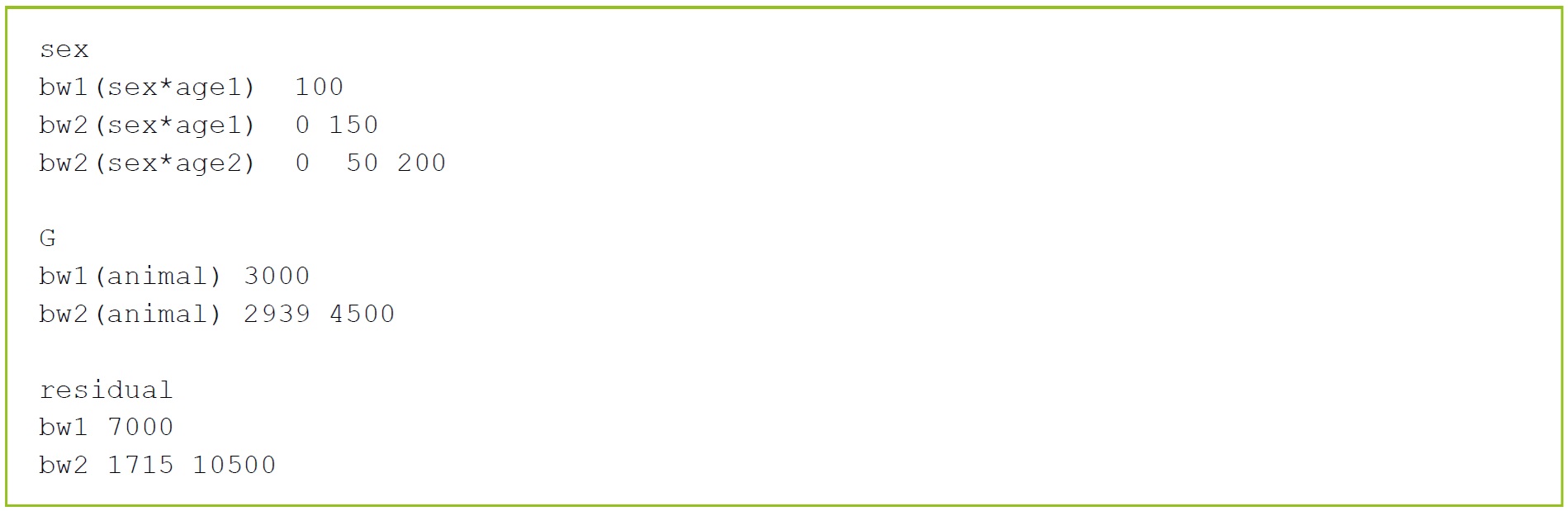
Example. The lower triangular trait (co)variance components file with two traits (body weight 1 and body weight 2) for non-genetic random regression, animal genetic and residual effects.

6.1.3. Input file in sparse-matrix format for the MiX99 solver

In the sparse matrix form, the order of the matrices must be the same as the order of random effects in the model, with the restriction that the genetic effect should be the last random effect in the model and the elements of its (co)variance matrix should appear in the sparse matrix file just before the elements of the residual (co)variance matrix. The residual (co) variance matrix should be specified at the end of the sparse matrix file. In summary, the order of matrices is: * Non-genetic random effects in the same order as specified in the model * Genetic effects as specified in the model * Residual effect The matrix elements must be specified as the random effect number, row number, column number and the value of the (co)variance. To avoid mistakes, it is recommended to provide the elements of the lower triangle of the matrix, in other words, any column number is smaller than or equal to the row number. Off-diagonals only need to be specified if they are non-zero. When haplotypes are used in the model for marker-assisted BLUP with the use of an inverse IBD matrix, both haplotypes are counted as effects, but the same variance components are used for the first and the second haplotype, when haplotypes are combined with the AND function, so the variance components should not be repeated for the second haplotype. Effectively, the effect number corresponding to the second haplotype is skipped from the list of inverse matrix elements. See Example 5.4 in the Appendix.

Example. The trait (co) variance components file in sparse-matrix format with two traits for the animal genetic and residual effects Columns: random effect number, trait row number, trait column number and variance or covariance component.

6.1.4. Syntax

PARFILE <filename> [!SPARSE]

Qualifier:

!Sparse
If !SPARSE is specified, the variance and covariance components are read in sparse matrix form. If omitted, the matrix is read in lower triangular form.

6.2. Parameter files for general covariates

6.2.1. General

The regression parameter file is specified for each general covariate file that is fitted as random regression. The file may contain a single set of variances and covariances between traits that apply to all covariates or a set for each covariate separately. The MiXBLUP shell checks whether scaling is necessary to avoid an error that the matrix is not positive-definite and applies any required scaling automatically. For the hpblup solver, the repression parameter file is provided as an inverse.

6.2.2. Input file

The format of the files with parameters of general covariates is the lower-triangular-matrix format of the general parameter file. For the MiX99 solver, every line of the variance covariance matrix starts with the trait name, as it is used in MiXBLUP instruction file. Note that trait names are case-sensitive. If !RegType R is specified for the covariate file, a single trait-effect variance-covariance matrix can be used for all covariates in the file. If !RegType H is used, a trait-effect variance-covariance matrix has to be specified for each covariate.

Example. Regression parameter file with a single set of variances and covariances between traits for all covariates. A regression parameter with covariate-specific variances and covariances contain such a set for each covariate. The number in the label of the matrix is linked with the position of the covariate in the record.

For the hpblup solver, a general covariate file may be fitted for multiple indices, so it is necessary to specify the trait name followed by the index name between brackets at the start of each line in the variance covariance matrix. If !RegType H is used, a trait-effect variance-covariance matrix has to be specified for each covariate.

Example. Regression parameter file with a single set of variances and covariances between traits for all covariates, for the hpblup solver.

6.2.3. Syntax

REGPARFILE REG01 <file name REG01>
REG02 <file name REG02>
<...>
REG99 <file name REG99>

REGPARFILE
The REGPARFILE section must contain the name of a parameter file for each covariate file for which the covariates are fitted as a random regression (so !REGTYPE is either ‘r’ or ‘h’). If the regression type is fixed, the corresponding file in REGPARFILE is ignored. The REGPARFILE section does not have any associated qualifiers. The lines of the REGPARFILE section each contain two columns. The first column is the label that links the parameter file to the covariate file. The second column is the name of the file.

6.3. Parameters for SNP covariate files

6.3.1. General

The SNP parameter file is specified for SNP covariate files that are to be fitted for random regression. The file may contain a single set of variances and covariances between traits for all SNP covariates or a set for each SNP covariate separately. For a SNPBLUP model without a direct genetic effect and SNP genotypes presented as 0, 1 and 2, the SNP variance can be calculated from the direct genetic variance with

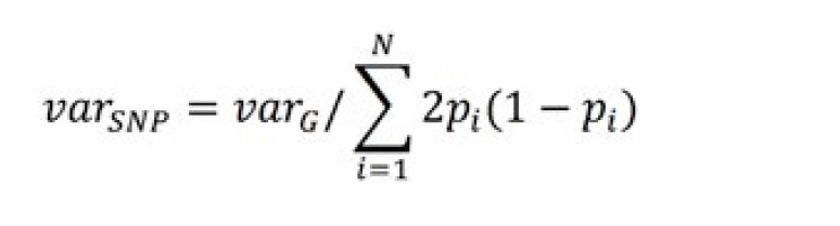
where N is the number of informative SNPs and pi is the allele frequency of the SNP allele counted on locus i. Non-informative SNPs must not be included in this calculation. If variances smaller than 1.0E-06 are specified, then the MiXBLUP kernel may give an error that the variance-covariance matrix is not positive-definite. This can be resolved by scaling the phenotypes with 10 or 100 and the variances with 100 or 10,000 accordingly. The MiXBLUP shell checks whether scaling is necessary and applies any required scaling automatically.

6.3.2. Input file

The format of the files with parameters of SNP covariates is the lower-triangular-matrix format of the general parameter file. If a single set of variances and covariances between traits is to be used for all SNP covariates (so !REGTYPE is ‘r’), then only one matrix needs to be specified. The matrix label needs to start with ‘SNP’, but the number is ignored. If SNP-specific variances and covariances are to be used (so !REGTYPE is ‘h’), then a matrix has to be specified for every SNP covariate separately. Depending on the number of SNP covariates in a file, this could be many thousands. The label has to start with ‘SNP’. The number in the label of the matrix is linked with the position of the SNP covariate in the record of the corresponding file. The number must be sequential and may be an integer between 1 and 2.1 billion. The label of a matrix in a SNP parameter file refers to a SNP covariate in the corresponding covariate file and should not be confused with the label linking the SNP covariate and parameter files. For the MiX99 solver, every line of the variance covariance matrix starts with the trait name, as it is used in MiXBLUP instruction file.

Example. SNP parameter file with a single set of variances and covariances between traits for all SNP covariates, for the MiX99 solver.

For the hpblup solver, a SNP covariate file may be fitted for multiple indices, so it is necessary to specify the trait name followed by the index name between brackets at the start of each line in the variance covariance matrix.

Example. SNP parameter file with a single set of variances and covariances between traits for all SNP covariates, for the hpblup solver.

6.3.3. Syntax

SNPPARFILE
SNP01 <file name SNP01>
SNP02 <file name SNP02>
<...>
SNP99 <file name SNP99>

SNPPARFILE
The SNPPARFILE section specifies the name of a parameter file for each SNP covariate file for which the SNP covariates are fitted as a random regression (so !REGTYPE is either ‘r’ or ‘h’). If the regression type is random and !CalcSNPvar has been specified, the corresponding file in SNPPARFILE is ignored. The SNPPARFILE section does not have any associated qualifiers. The lines of the SNPPARFILE section each contain two columns. The first column is the label that links the parameter file to the SNP covariate file. The second column is the name of the file.

6.4. Parameters in case of heterogeneous residual variances

6.4.1. General

The residual variance may not be the same for all observations. If this is the case, observations can be grouped by their residual variance prior to the analysis. A column in the data file links the observation to the correct residual variance matrix. Modelling data with a random regression approach often requires the use of multiple residual variance classes.

6.4.2. Input file

The file contains a matrix for every class number in the linking column in the data file. The name of the matrix is Res followed by the class number between brackets. The class number has to be an integer. The example below gives the series of residual matrices for a situation with observations being linked to one of three residual variances classes.

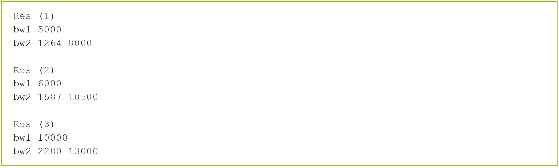
Example. The residual covariance file with three residual variance-covariance matrices.

6.4.3. Syntax

DATAFILE <filename>
\<...>
[<field j> I !RESVARCLASS]
<..>
RESFILE <filename>

Section:

RESFILE
The RESFILE section specifies the name of the file with residual between-trait variance-covariance matrices. The RESFILE section does not have specific qualifiers.

Qualifier:

!RESVARCLASS
The qualifier !ResVarClass in the DATAFILE section links a data record to the appropriate residual variance class, in case the residual variance differs for groups of records. The field is integer. The qualifier !RESVARCLASS must be used if the section RESFILE is specified.

7. Statistical models

Observed traits on two individuals may be similar due to genetic effects and systematic non-genetic effects. The statistical model contains all such effects known to explain variation in observed traits. This chapter describes various statistical models to estimate genetic effects on traits with as little bias as possible.

7.1. Basic models

7.1.1. General

The MODEL section specifies the start of the statistical models for the traits in the analysis. Traits and statistical models start immediately below the line with the MODEL keyword. For each trait, the statistical model is specified on a separate line. MiXBLUP supports up to 63 traits to be analysed simultaneously, if computer resources permit this. The basic statistical model for a breeding value evaluation contains fixed effects, uncorrelated, non-genetic random effects and a direct genetic random effect. Uncorrelated, non-genetic random class effects are assumed to have an identity relationship matrix between levels of the effect. Each model line contains trait name, fixed effects, non-genetic random effects and genetic random effects. Fixed effects may be class effects, covariates or covariates nested within a class effect. Similarly, random effects may be class effects or covariates nested within a class effect. The residual random effect does not need to be specified. The minimum statistical model contains one fixed effect and one genetic random effect.

7.1.2. Syntax

MODEL
<trait1> ~ <class effects> [covariates] [class effect * covariates] &!RANDOM G(<direct genetic effect>) [<non-genetic random effects>]
[<trait2> ...]
<...>
[ ...]

Section:

MODEL
The MODEL section specifies the statistical model for the traits in the analysis.

Qualifiers:

\~ (tilde)
The tilde separates the trait from the statistical model.

* (star)
The star is used for nesting a covariate within a class effect, to yield a regression coefficient for each level of the class effect. This can be used for both fixed and random nested covariates. The star must not be used to model an interaction of class effects.

!RANDOM
The !RANDOM qualifier separates the fixed effects from the random effects in the model.

G(...)
The G(...) function links a random effect to the inverse genetic or genomic relationship matrix.

7.1.3. Associated output files

Output file	Description
Solfix.txt	Solutions of fixed effects by trait (class effects, covariates and nested covariates)
Solfix.out	As Solfix.txt, but for alphanumerical class labels
Solr00.txt	Solutions of non-genetic, uncorrelated random effect 00 by trait, where 00 ranges
	from 1 to the number of non-genetic, uncorrelated random effects across traits
	(class effects, covariates and nested covariates)
Solr00.out	As Solr00.txt, but for alphanumerical class labels

7.2. Repeatability models

7.2.1. General

Certain traits are measured just once in the lifetime of an individual. Other traits may be measured repeatedly. Two observations on a single individual are more similar than expected from having the same genotype. A permanent environmental effect is usually added to the model to account for non-genetic similarity of records of the same individual. Such a permanent environmental effect has the same label as the direct genetic effect, but with an identity relationship matrix between levels. This permanent environmental effect should have its own column in the data file and must not be the column with the direct genetic effect (although identical).

7.2.2. Syntax

MODEL
<trait\1> ~ \<fixed effects> !RANDOM G(<direct genetic effect>) <permanent environmental effect>
<...>
[<traitN> ...]

7.2.3. Associated output files

Output file	Description
Solr00.txt	Solutions of non-genetic, uncorrelated random effect 00 by trait, where 00 ranges
	from 1 to the number of non-genetic, uncorrelated random effects across traits
	(among which the permanent environmental effect)
Solr00.out	As Solr00.txt, but for alphanumerical class labels

7.3. Maternal genetic models

7.3.1. General

Some traits are affected by the genotype of the animal itself and the genotype of its dam at the same time. An example is weaning weight in beef cattle. For such traits, a maternal genetic model should be used. The inverse numerator relationship matrix is applied both to the direct genetic effect (animal) and the maternal genetic effect (dam). The maternal genetic effect must be a separate field in the data file and each individual in this field must exist as an individual in pedigree, genotype file or other resource of genetic similarity. For biological dams, this is self-evident, but for foster dams, this requires special attention.

7.3.2. Syntax

MODEL
<trait\1> ~ \<fixed effects> !RANDOM <...> G<direct genetic effect>, <maternal genetic effect>)
<...>
[<traitN> ...]

The maternal genetic effect is placed within the brackets of function G to link it with the relationship matrix between individuals.

7.3.3. Associated output files

Output file	Description
Solani.txt	The solutions of the maternal genetic effect are included as additional columns in
	Solani.txt. The exact layout of Solani.txt is printed at the end of solver.log.
Solani.out	As Solani.txt, but for alphanumerical ID labels

7.4. Social interaction models

7.4.1. General

The social interaction model (or group selection) is used to estimate the effects of an individual’s genotype on its own performance and on the performance of its pen mates simultaneously. It should be used for groups of a single group size, but a slightly varying group size is also supported. For a single group size, a genetic effect for social interaction is fitted for each pen mate. This effect can be interpreted as the genetic value for supporting or inhibiting the expression of the direct genetic merit of pen mates. The genetic variance of this social effect is dependent on the size of the group, so performance in small and large groups by design should not be combined as one trait. If the size of groups is the same by design, but it varies slightly due to death or removal from the pen, it is still possible to fit a social interaction model by adding a covariate of either 0 (not present) or 1 (present) and apply a nested regression of this covariate within pen mate. The ID label used for not-present pen mates must appear in the pedigree or genotype file, too, but no information is added to its social genetic value when the covariate is zero (not present).

7.4.2. Syntax of the social interaction model with one group size for all groups for the MiX99 solver

DATAFILE
<ID individual> <field type I or A>
<...>
mate1 I
mate2 I
<...>
mateN I
MODEL
<trait1> ~ <...> !RANDOM <...> G(<ID individual>,mate1 AND mate2 <...> AND mateN)
[<trait2> ...]
<...>
[<traitN> ...]

The pen mates need to be defined in the data file. The number of additional columns is equal to the number of pen mates (mate1, mate2, ..., mateN).

Qualifier:

AND
The function AND combines the effects of different mates to one design matrix. There are a few constraints when combining effects; all of them are rare:

• When ‘AND’ is used for group selection, it cannot be used for IBD-haplotypes. In other words, haplotype effects cannot be included in a social interaction model.
• Combining of effects needs to be the same for any traits for which effects are combined. In other words, traits measured when the animal was in a different group need to be analyzed in a separate analysis.
• The parser supports an evaluation in which some traits have social genetic effects and other traits do not.
• There can be only one group of combined genetic effects, so no commas must be placed between the effects of mates. It means that the genetic effects can only be combined to one other effect and not more.
• The order of genetic effects should be kept the same across traits with a social interaction model.

7.4.3. Syntax of the social interaction model with slightly varying group sizes for the MiX99 solver

DATAFILE
<ID individual> <field type I or A>
<...> mate1 I
present1 R
mate2 I
present2 R
\<...>
mateN I
presentN R
MODEL
<trait1> ~ <...> !RANDOM <...> G(<ID individual>,present1*mate1 AND present2*mate2 <...> AND presentN*mateN)
[<trait2> <...>]
<...>
[<traitN> <...>]

Both the pen mates and their presence need to be defined in the data file. The number of additional columns is therefore equal to two times the number of pen mates (mate1, mate2, ..., mateN, present1, present2, ..., presentN).

7.4.4. Syntax of the social interaction model for the hpblup solver

DATAFILE
Animal I
<...>
mate1 I
mate2 I
<...>
mateN I
MODEL
<trait1> ~ <...> <...> !RANDOM <...> G(Animal,LINK(mate1))
[<traitN> <...>]
LINKEDEFFECTS
mate1 ~ mate2 ... mateN

The pen mates need to be defined in the data file. The number of additional columns is equal to the number of pen mates (mate1, mate2, ..., mateN). For slightly varying group sizes, just use a zero for a missing pen mate.

Section:

LINKEDEFFECTS
The section LinkedEffects is used to specify which effects are linked to the leading effect and should be combined with the leading effect. The leading effect should be presented before the tilde (~); linked effects should be presented after it. The number of lines in the LinkedEffect section matches the number of unique occurrences of the LINK function in the MODEL section. So if multiple traits contain G(Animal,LINK(mate1)) in the model, only one line is needed in the LinkedEffect section.

Qualifier:

LINK
The function LINK specifies the leading effect of a set of linked effects in the model.

7.4.5. Associated output files

Output file	Description
Solani.txt	The solutions of the social genetic effects are included as additional columns in
	Solani.txt. The exact layout of Solani.txt is printed at the end of solver.log.
Solani.out	As Solani.txt, but for alphanumerical ID labels

7.5. Random regression models

7.5.1. General

There are two types of random regression models supported by MiXBLUP, the non-genetic and genetic random regression model. Both original covariates and polynomials derived from an independent variable may be used in the model. In a non-genetic random regression model, the regression of the observations on an independent covariate is fitted as a random effect. Random regression in MiXBLUP has to be specified as regression nested within a class variable. If no nested regression is required, the user needs to add a column of ones to the data file, and fit the covariate within this class effect of a single level. The internal structure of MiXBLUP requires that any random effect be associated with a class effect. This can be seen in the parameter files, too, where variance-covariance matrices are all specified by class effect. In a genetic random regression model, trait observations are regressed on the covariate within animals, taking into account the genetic relationships between animals. The estimated breeding values from such an analysis concern the animal-specific parameters of the line or curve fitted. The user needs to convert these estimates to estimated breeding values at a given level of the covariate or for a function of levels of the covariate. If the relationship between an observed trait and an independent variable is non-linear, it may still be possible to model the relationship with polynomials, as a special case of multiple linear regression. Polynomial regression is a form of linear regression in which the relationship between the independent variable x and the observed trait is modelled as an nth degree polynomial in x by fitting (n+1) covariates derived from x. Polynomials may be provided by the user either in the data file or in a covariate table, or may calculated during the preparations for the analysis and stored in a covariate table. Polynomials calculated by MiXBLUP are Legendre polynomials.

7.5.2. Syntax of a simple non-genetic random regression model for the MiX99 solver

MODEL
<trait1> ~ <...> !RANDOM <class>*<covariate> [<class>*<covariate> <...>]
<...>
[<traitN> <...>]

The random regression term consists of a class effect with field type integer (I) or alphanumerical (A) and a covariate with field type real (R). Each random regression term has to be present in the variance-covariance matrix of the class effect in the parameter file (see chapter 6.1.).

Qualifier:

* (star)
The star is used for nesting a covariate within a class effect, to yield a regression coefficient for each level of the class effect. There is no specific order of class effect and covariate in the term.

7.5.3. Syntax of a simple genetic random regression model for the MiX99 solver

MODEL
<trait1> ~ <...> !RANDOM G(<ID>*<covariate>[,<ID>*<covariate>]) <...>
<...>
[<traitN> <...>]

The regression terms nested within the individual’s ID are placed within the function G(...) to indicate that the relationship matrix of individuals should be used.

7.5.4. Syntax of a polynomial regression model using a covariate table for the MiX99 solver

CVRTABLE <name covariate>
MODEL
<trait1> ~ <...> <class>*CVR(<n1>) !RANDOM <class>*CVR(<n2>) G(<ID>*CVR(<n3>)) <...>
<...>
[<traitN> <...>]

For the use of covariate table files with the MiX99 solver, see chapter 4.2.2.1. and 4.2.2.3..

Qualifier:

CVR(...)
The CVR function is used in the MODEL section and is a shorthand for all polynomial terms to be fitted and may be used in the same way as any individual random regression term. The alternative way to specify polynomial random regression is to use the individual columns of the covariate table file. The names of the columns are cvr00, cvr01, cvr02, ..., cvrnn. The label is lowercase and has exactly two digits ranging from 00 to 99.

7.5.5. Syntax of a simple non-genetic random regression model for the hpblup solver

REGFILE
<field ID> <field type I or A>
REG02 <file name REG02> !REGTYPE <R or H>
REGPARFILE
REG02 <file name REG02>
MODEL
<trait1> ~ <...> !RANDOM <class>*hpReg(<field ID>,2) [<class>*hpReg(<field dam ID>,2) <...>]
<...>
[<traitN> <...>]

For the hpblup solver, covariates in a random regression should be provided in a covariate table or a general covariate file, but not as a field in the data file. The random regression term consists of a class effect with field type integer (I) or alphanumerical (A) and a covariate with field type real (R). Each random regression term has to be present in the variance-covariance matrix of the class effect in the parameter file (see chapter 6.1).

Qualifier:

* (star)
The star is used for nesting a covariate within a class effect, to yield a regression coefficient for each level of the class effect. There is no specific order of class effect and covariate in the term.

7.5.6. Syntax of a simple genetic random regression model for the hpblup solver

REGFILE
<field ID> <field type I or A>
REG02 <file name REG02> !REGTYPE <R or H>
REGPARFILE
REG02 <file name REG02>
MODEL
<trait1> ~ <...> !RANDOM G(<ID>*hpReg(<field ID>,2)) <...>
<...>
[<traitN> <...>]

For the hpblup solver, covariates in a random regression should be provided in a covariate table or a general covariate file, but not as a field in the data file. The regression terms nested within the individual’s ID are placed within the function G(...) to indicate that the relationship matrix of individuals should be used.

7.5.7. Syntax of a polynomial regression model using a covariate table for the hpblup solver

CVRTABLE !nCVRTABLES 2
TABLE01 <filename> !CVRNUM <nth order> !CVRMIN <minimum value> !CVRMAX <maximum value> !CVRSingleCov !CVRIndex <index field name>
TABLE04 <filename> !CVRNUM <nth order> !CVRMIN <minimum value> !CVRMAX <maximum value> !CVRSingleCov !CVRIndex <index field name>
MODEL
<trait> ~ <fixed effects> <Class1>*TABLE01 !RANDOM <Class2>*TABLE04 G(Animal*TABLE04)

For the use of covariate table files with the hpblup solver, see chapter 4.2.2.2. and 4.2.2.4..

Qualifier:

TABLEnn
The TABLEnn label is a shorthand for a specific covariate table file. It automatically fits all covariates in the file, unlike for the CVR(...) function for the MiX99 solver, which can be used to fit a smaller number of covariates from a covariate table file. The names of the covariates in the parameter file with trait variance-covariance matrices are TABLEnn_cc, where nn is the table number and cc the covariate number starting with 00 (for example TABLE01_00 for the first covariate).

7.5.8. Associated output files

Output file	Description
Solani.txt	The solutions of the genetic nested regression effects are included as additional
	columns in Solani.txt. The exact layout of Solani.txt is printed at the end of solver.log.
Solani.out	As Solani.txt, but for alphanumerical ID labels
Solr00.txt	The solutions of the non-genetic nested regression effects are included as
	additional columns in Solr00.txt. The exact layout of Solr00.txt is printed at the end
	of solver.log.
Solr00.out	As Solr00.txt, but for alphanumerical class labels

7.6. Weighting residuals by record

7.6.1. General

If the common assumption of constant standard deviation of the residuals (i.e. homogeneous residual variance) is not met, it is possible to weight individual records. Less precise measurements get less weight and more weight is given to more precise measurements when estimating breeding values. An example is the use of de-regressed breeding values as a pseudo-phenotype. The standard deviation of the residual depends on the reliability of the original estimated breeding value. A weighting factor based on the reliability can be used to give more weight to pseudo-phenotypes based on a relatively large amount of information. Another example is variation in residual variances within contemporary groups. Observations in contemporary groups with a large residual variance can be given a proportionally lower weighting factor.

7.6.2. Syntax

MODEL
<trait1> [!WEIGHT <weighting factor>] ~ <fixed effects> !RANDOM G(<ID>) [<non-genetic random effects>]
<...>
[<traitN> <...>]

Qualifier:

!WEIGHT
A field in the data file can be specified as a weighting factor for a specific trait using the !WEIGHT qualifier.

7.6.3. Associated output files

The standard output files are used for a weighted analysis.

7.7. Combining effects across traits

7.7.1. General

If a trait measured in different cycles or parities or on individuals of different strains and crosses is modelled as multiple traits, it may be desirable to estimate fixed effects across these traits, in order to increase the precision of the solutions of the model. Random effects can easily be combined by specifying covariances between the traits that are equivalent to a correlation close to unity. For fixed effects, it has to be specified across which traits the effect should be estimated.

7.7.2. Syntax

MODEL
<trait1> ~ <fixed1> !RANDOM G(<ID>) [<random1>]
<trait2> ~ <fixed1> !RANDOM G(<ID>) [<random1>]
<...>
<traitN> ~ <fixed> !RANDOM G(<ID>) [<random>]
COMBINE
<fixed1> ~ <trait1> <trait2>

Section:

COMBINE
The section COMBINE allows to specify across which traits a fixed effect should be estimated. It supports class effects, covariates and nested covariates.

7.7.3. Associated output files

The standard output files are used for an analysis with fixed and random effects estimated across several traits.

7.8. Correction of heterogeneous residual variances

7.8.1. General

If residual variance within contemporary groups varies (heterogeneous residual variance), the user may specify appropriate weighting factors in the data file and weight records accordingly (see chapter 7.6.). MiXBLUP also offers the possibility to calculate appropriate weighting factors in a three-step approach. In the first step, the traits are analysed with the assumption of homogeneous residual variance. The residuals (ê) are read from the output of step 1 and the linearized squared residuals (z) for trait i and animal j are calculated as

Var(e~i~) is the residual variance of trait i used in the first step and is obtained from the res(idual) matrix in the parameter file or, if residual variance classes are used, the residual variance of the corresponding class of the record. In the second step, these linearised squared residuals are analysed using a suitable model. The predicted phenotypes of this second model are used to calculate weighting factors. The weighting factor for trait i and individual j is calculated from the predicted value of the linearised squared residual (Z~ij~) as

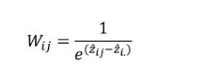
where Z~i.~ is the average predicted value of the linearized squared residual for trait i across all individuals. In the third step, the analysis of the first step is repeated, but with a weighting factor added to account for heterogeneous residual variance. MiXBLUP can run these three steps in a single process.

7.8.2. Syntax

MODEL
<trait1> ~ <fixed1> !RANDOM <random1> G(<ID>)
<trait2> ~ <fixed2> !RANDOM <random2> G(<ID>)
<trait3> ~ <fixed3> !RANDOM <random3> G(<ID>)
VARMODEL
LSR1 ~ <fixed> !RANDOM <random> G() !VARTRAIT <trait1> LSR2 ~ <fixed> !RANDOM <random> G(<ID>) !VARTRAIT <trait2>
SOLVING
!DHGLM !HETCOR

Section:

VARMODEL
The VARMODEL section specifies the statistical model for the second step for the linearized squared residuals.

Qualifiers:

!VARTRAIT
The qualifier !VARTRAIT in the VARMODEL section is mandatory and links the linearized squared residual to the original trait. Original traits do not have to be all represented in the VARMODEL section.

!DHGLM
The option !DHGLM in the SOLVING section prepares MiXBLUP for multiple calls of the kernel.

!HETCOR
The qualifier !HETCOR in the SOLVING section creates the data file and instruction file for each step.

7.8.3. Associated output files

The standard output files are used for an analysis with correction for heterogeneous variances.

7.9. Using a threshold model for a categorical trait (MiX99 solver only)

7.9.1. General

The linear model used in MiXBLUP to estimate breeding values is based on the assumptions that a trait has a continuous normal distribution, its components of variance are homogeneous and residuals are uncorrelated with genetic and non-genetic random effects. There are traits that are recorded as categories. A binary trait has only two possible categories, for example, present or absent, true or false, all or none. Traits with more than two categories may be ordered, for example small-medium-large, or unordered, such as red-yellow-blue. For categorical traits, the usual assumptions of a linear model are violated.

It has been proposed to overcome this by assuming a continuous trait underlying the categorical trait. Thresholds on the underlying scale determine the recorded category on the observed scale. The threshold model is more demanding than the linear model. There are methods available for the threshold model: Newton-Raphson (NR) and Expectation-Maximisation (EM). Both methods give the same results but use a different route. Both methods have two levels of iterations. The outer level iterates on the thresholds, given the set of estimated solutions of the previous iteration. The inner level iterates on the solutions given the current estimates of the threshold. Currently only one categorical trait can be analysed with a threshold model in a multi-trait evaluation of any number of traits analysed with a linear model. Although theoretically incorrect, assuming a linear model for a categorical trait often yield solutions that rank selection candidates largely in correct order. This is especially the case for intermediate prevalence of categories.

7.9.2. Input files

Category labels must be numbered 1 to the number of categories for the MiXBLUP kernel. MiXBLUP can rename category labels for this purpose from a file with ordered labels by trait. The file is specified with !CONVERTCAT. The first field is the trait name in the data file. Subsequent fields contain the category labels. The position in the sequence determines the new sequential integer code, 1..n. Although MiXBLUP currently supports only a single trait with a threshold model in combination with any number of traits with a linear model, multiple traits may be specified for use across evaluations. In the example below, the stature categories Small, Medium and Large are converted to 1, 2 and 3, according to their positions in the record. The diseased categories 1 and 0 are converted to 1 and 2. Note that a binary trait coded as 0/1 has to be converted to 1 and 2.

Stature Small Medium Tall
Diseased 1 0

Example. Category conversion table.

It is also possible to fix thresholds at a predefined value, using !THRFIXED. Thresholds must be taken from a N(0,1) underlying distribution. The file may contain any number of categorical traits, but in any evaluation, only one categorical trait can be analysed with a threshold model, currently. The number of thresholds to be specified is the number of categories minus 1. Thresholds may be taken from a previous analysis or calculated from the observed prevalence in a larger set of data.

Stature -0.34 0.56
Diseased 0.0

Example. Table with fixed thresholds.

7.9.3. Syntax

DATAFILE <filename> [!CONVERTCAT <filename>]
<...>
MODEL
<trait1> ~ <fixed1> !RANDOM <random1> G(<ID>)
<...>
<trait3> ~ <fixed3> !RANDOM <random3> G(<ID>) !THRESHOLD <number of thresholds>
SOLVING
[!THRMAXIT <maximum number of NR or EM iterations at outer level>] [!THRMAXPCG <maximum number of iterations at inner level>]
[!THRMETHOD <EM or NR>]
[!THRFIXED <filename>]

Qualifiers:

!CONVERTCAT
The qualifier !CONVERTCAT in the DATAFILE section is optional. It can be used to specify a file with category labels.

!THRESHOLD
The option !THRESHOLD in the MODEL section is mandatory and specifies which trait is to be analysed with a threshold model.

!THRMAXIT
The qualifier !THRMAXIT in the SOLVING section can be used to specify the maximum number of NR or EM iterations. The default number is 5,000.

!THRMXPCG
The qualifier !THRMAXPCG in the solving section is optional and specifies the maximum number of iterations within each NR or EM iteration. The default number is 100.

!THRMETHOD
The qualifier !THRMETHOD is optional and specifies the method to implement the threshold model. The default method is NR. The alternative method is EM.

!THRFIXED
The qualifier !THRFIXED is optional and can be used to specify a file with fixed thresholds per trait.

7.9.4. Associated files

The standard output files are used for an analysis with a threshold model.

8. Control of analysis and output

This chapter describes the control part of the instruction file, which can be used to control the analysis and the output generated from the analysis.

8.1. Control of the analysis

8.1.1. General

Control of an iterative process like solving a linear system to estimate breeding values involves setting the convergence criterion and the maximum number of iterations, specifying whether the run is a continuation or a new start and defining the starting values for a new evaluation. An more advanced option is to specify the type of preconditioner to be used for solving the system. Generally, the default type of preconditioner is optimal. The default varies across models to specify genetic similarity between individuals.

8.1.2. Syntax

8.1.2.1. Syntax when using MiX99 solver

SOLVING
[!MAXIT <number of rounds>]
[!STOPCRIT <convergence criterion>]
[!NOPEEK]
[!PEEKFIRST <iteration number>]
[!PEEKEVERY <number of rounds>]
[!PEEKKEEP]
[!RESTART]
[!GFROMDISK]
PRECON <n, b, d>
[!WITHINBL <b, d>]
[!ACROSSBL <f, m, b, d>]

Sections:

SOLVING The SOLVING section is used to control the process and the output of the analysis.

PRECON <option> The PRECON section can be used to change the type of preconditioner. Possible options are n (no preconditioner), b (block-diagonal preconditioner) and d (diagonal preconditioner).

Qualifiers:

!MAXIT <number of iterations> The optional !MAXIT qualifier in the SOLVING section can be used to set the maximum number of iterations to be used. If !MAXIT is not specified, the default maximum number of iterations is 5,000.

!STOPCRIT <convergence criterion> If the convergence criterion needs to be different from 1.0E-04, it can be set with the optional !STOPCRIT qualifier in the SOLVING section.

!NOPEEK MiXBLUP stores intermediate results by default every 100th iteration. All solutions files are created and starting values for a restart are stored as if solutions have converged. By default, only the last set of preliminary results is kept. The name of each of the file is the normal file name extended with _PEEK, so for example Solani_PEEK.txt and solunf_PEEK. The last set of preliminary results will be removed when convergence has been attained or the maximum number of iterations reached The process of storing preliminary results can be avoided by specifying !NOPEEK.

!PEEKFIRST <iteration number> The iteration number at which the preliminary results are stored for the first time can be specified with !PEEKFIRST.

!PEEKEVERY <number of iterations> The number of iterations between storing two subsequent sets of preliminary results can be specified with !PEEKEVERY.

!PEEKKEEP Instead of only keeping the last set of preliminary results, MiXBLUP can also retain each set of preliminary results. In this case, the name of each file is the normal file name extended with the iteration number, so for example Solani_100.txt and solunf_100.txt. This option can be specified with !PEEKKEEP. This option is useful for investigating the causes of unexpected convergence behaviour.

!RESTART The optional qualifier !RESTART can be used to specify that preliminary solutions of an interrupted analysis or old solutions of the previous analysis are to be used as starting values for the new evaluation. This option links old solutions to class effect levels using the coded labels.

!GFROMDISK The !GFROMDISK qualifier instructs the solver to read the inverse genomic relationship matrix from disk during solving. This was the only option in previous versions of MiXBLUP. The new default is to keep this matrix in memory, which is more demanding for memory requirement, but it saves the time to read this matrix every iteration.

!WITHINBL <option> The optional qualifier !WITHINBL is used in the PRECON section and can be used to use a different preconditioner for the within-block effects than the default preconditioner type. Valid options are b (block-diagonal) and d (diagonal).

!ACROSSBL <option> The optional qualifier !ACROSSBL is used in the PRECON section and can be used to use a different preconditioner for the across-block effects than the default preconditioner type. Valid options are f (full), m (mixed), b (block-diagonal) and d (diagonal).

8.1.2.2. Syntax when using hpblup solver

SOLVING
[!hpblup]
[!hpCriterion <type of convergence criterion>]
[!NumProc <number of cpu>]
[!MAXIT <number of rounds>]
[!STOPCRIT <convergence criterion>]
[!STARTVAL_CHECK]
[!MIRACULIX]
[!MIRACULIX_GPU]
[!NOPEEK]
[!PEEKFIRST <iteration number>]
[!PEEKEVERY <number of rounds>]
[!PEEKKEEP]

Additional qualifiers:

!hpblup This qualifier is used to triggers MiXBLUP to call the hpblup solver instead of the default MiX99 solver

!hpCriterion This qualifier is used to specify the convergence criterion to be used, ck, cr or cd (default).

!STARTVAL_CHECK The optional qualifier !STARTVAL_CHECK only applies to the hpblup solver and links old solutions to class effect levels using the original class effect labels. Compared to the !RESTART option, the !STARTVAL_CHECK option will do an extra step of decoding class effect levels of old solutions and re-coding them given the new set of data. The !RESTART option can be used for the hpblup solver, but old solutions will be linked to incorrect class effect levels if any previously used class effect levels with a solution are no longer present. In that case, solutions are still correct, provided that they have converged, but it takes more iterations to obtain them than using the correct old solutions as starting values.

!NumProc This qualifier is optional and can be used to specify the number of cpus to be allocated to hpblup. This number has to be equal to or lower than number available for the evaluation.

For the meaning of the other qualifiers, see previous chapter.

8.2. Control of output

8.2.1. General

A successful analysis produces at least a log file and files with solutions to all effects in the model. In some cases, additional results may be required for development or evaluation purposes. Various options are available to specify these additional files when required.

8.2.2. Syntax

8.2.2.1. Syntax when using MiX99 solver

SOLVING
[!BASEANIMALSZERO <filename>]
[!YHAT]
[!EHAT]
[!YIELDDEV]
[!IDD]
[!DYD]
[!KEEPTMP]
[!SELINDEX <filename>]
[!FILTER \]
TMPDIR <work directory>

Sections:

TMPDIR The TMPDIR section can be used to specify an existing folder to store the temporary files of the kernel.

Qualifiers:

!BASEANIMALSZERO <filename> The estimated breeding values of each individual in Solani.txt or Solani.out can be presented as a deviation of a genetic base, which is the average of a specified group of individuals, which are referred to as base animals. The ID of the base animals should be given in the specified file, or in BaseAnimals.dat. The file should contain one ID per row. The average per trait of the group of base animals is included in the log file MiXBLUP.log. If not all individuals are present in the data file, then a warning is given in the log file MiXBLUP.log. The specified file BaseAnimals.dat should contain the original IDs as they appear in the pedigree file.

!YHAT The optional qualifier !YHAT creates a prediction for each observed trait and each animal in the data file. The predictions are stored in Yhat.txt, which is a text file that contains the animal ID in the first column and predicted observations for each trait in the model in subsequent columns. Missing observations in the data file get the code -8192.0 in the file with predictions.

!EHAT The optional qualifier !EHAT stores the residual term of each observed trait and each animal in the data file. The residuals are stored in Ehat.txt, which is in text format and contains the animal ID in the first column and residuals for each trait in the model in subsequent columns. Missing observations in the data file get the code -8192.0 in the file with residuals.

!YIELDDEV The optional qualifier !YIELDDEV stores the observation corrected for fixed effects and non-genetic random effects for each observed trait and animal in the data file. The yield deviations are stored in YD.txt, which is in text format and contains the animal ID in the first column and yield deviations for each trait in the model in subsequent columns. Missing observations in the data file get the code -8192.0 in the output file.

!IDD The optional qualifier !IDD (“individual daughter deviation”) stores the yield deviation corrected for the genetic contribution of the dam for each observed trait and animal in the data file. The individual sire progeny deviations are stored in IDD.txt, which is in text format and contains the animal ID in the first column and yield deviations for each trait in the model in subsequent columns. Missing observations in the data file get the code -8192.0 in the output file.

!DYD The optional qualifier !DYD (“daughter yield deviation”) stores the individual yield deviations averaged by sire. The daughter yield deviations are stored in soldyd.txt, a text file that contains sire in the first column, the number of progeny included in the progeny yield deviation in the fourth column, the progeny yield deviations by trait followed by the same number of fields to indicate whether the progeny yield deviation of the corresponding trait is valid (value is 1) or not (value is 0).

!KEEPTMP The optional qualifier !KEEPTMP can be used to stop the removal of temporary files at the end of an analysis, for example to check for possible errors. The default is that all large temporary files are deleted as soon as they are no longer required.

!SELINDEX <filename> The qualifier !SELINDEX can be used to automatically calculate a selection index value as the sum of weighted genetic solutions (weighted EBV). The selection index value is added as an additional column in the Solani output file. The file specified after the qualifier contains the selection index weighting factor for each combination of genetic effect and trait in the model. The syntax is <trait>(<genetic effect>) <selection index weighting factor>, for example: phen1(animal) 1.0.

!FILTER <label> The qualifier !FILTER can be used to automatically prune the Solani output file. It can be used to include or exclude individuals from the solutions file. The pedigree file should contain a field either with the text <label> or something else. To exclude individuals marked with 'dead', use !FILTER <>dead. To include individuals born in 2025 only, use !FILTER 2025.

8.2.2.2. Syntax when using hpblup solver

SOLVING
[!BASEANIMALSZERO <filename>]
[!YHAT]
[!EHAT]
[!YIELDDEV]
[!KEEPTMP]
[!SELINDEX ]
[!FILTER \]
TMPDIR <work directory>

9. Reliabilities

Besides estimating genetic effects (or breeding values), MiXBLUP supports a second type of analysis to quantify the amount of information available to estimate the genetic effect of each individual. This is expressed as the reliability of the estimated (genomic) breeding value. This chapter describes how reliabilities can be calculated with MiXBLUP.

9.1. General

A reliability is a measure of the information that is available for the estimate of a breeding value. The reliability is dependent on the heritability and the presence of observations for the individual itself. The biggest impact on the reliability comes from the number of progeny with observations. Calculation of reliability is not supported for weighted residuals or marker haplotype models. Exact reliabilities can be calculated only for a relatively small number of individuals in the pedigree, say less than 100,000 individuals. Of these individuals, no more than say 40,000 individuals can have a genotype record. If there are more individuals in the evaluation, it is possible to calculate approximate reliabilities. Approximate reliabilities are built up from approximate pedigree reliabilities and the additional information provided by genomic relationships as a deviation from pedigree relationships.

MiXBLUP supports the calculation of an approximate or exact pedigree or genomic reliability of the EBVs of individuals for most statistical models.

Type of evaluation	Reliabilities	Remarks
Basic statistical model	direct	exact or approximate
Maternal genetic model	direct & maternal	exact or approximate
Social interaction model	direct & indirect	exact or approximate
Random regression model	direct	approximate; only for calculated totals
Pedigree relationships	direct & indirect	exact or approximate
Genomic relationships	pedigree + genomic	exact or approximate; requires hpblup
SNP covariates	pedigree + genomic	exact or approximate; requires hpblup

9.2. Exact reliabilities

1.1.1. General

Exact reliabilities are calculated from the prediction error variance of an estimate. Prediction error variance is obtained from the diagonal of the inverse of the coefficient matrix. The need of a full inverse limits the size of a dataset for which exact reliabilities can be calculated. A prediction error variance is available for each genetic and non-genetic solution of the evaluation. Reliabilities are available only for the solutions of genetic effects of individuals. Exact reliabilities are pedigree reliabilities if no genomic information is used and genomic reliabilities if it is used. Exact reliabilities and prediction error variances are only available for the hpblup solver.

9.2.1. Syntax

SOLVING
!hpblup
!reliab_exact

Qualifier:

!reliab_exact The !reliab_exact is used to specify the calculation of exact reliabilities for genetic effects and the prediction error variance for each solution in the analysis. It has to be used in tandem with !hpblup.

1.1.1. Associated output files

Output file	Description
aggregate_pev.dat	Prediction error variance of each solution
Relani.out	Reliabilities of genetic effects of individuals

9.3. Approximate reliabilities

9.3.1. General

Approximate pedigree reliabilities are calculated for families within blocks. It is a completely different process than estimating breeding values. Approximate reliabilities are calculated in a separate analysis.

1.1.1. The concept of blocks in the reliability calculation in MiXBLUP

9.3.1.1. Block variable

The calculation of reliabilities in MiXBLUP requires the use of a family block variable. The objective of using a block variable is to minimise the use of memory during the calculation by ordering of equations in equation family blocks (Lidauer and Strandén, 1999). Using a block variable has no benefit for breeding value estimation with MiXBLUP. To take advantage of this concept, it is important that each equation family block contains as many closely connected equations as possible, and that the number of equations connecting equation family blocks is as low as possible. A family consists of an individual, its parents and its progeny.

9.3.1.2. Common-block variable

Equations that connect all (or many) equations, such as individuals with progeny in many different blocks, can be grouped into one or several common blocks. Common blocks refer to blocks of equations, which will be kept in memory for all families. Equations of common blocks must be ordered to appear at the bottom of the MME, i.e. animals of common blocks must have largest block sorting variables. This ordering of mixed model equations yields for many animal breeding problems a structured coefficient matrix that has nearly doubly-bordered block diagonal form. The number of common blocks can be specified by the user. The default is that no common blocks are used. MiXBLUP will solve the mixed model equations even if such a structure cannot be achieved. However, pre-processing time may be longer than usual. As a consequence, it is important to keep this concept in mind when editing the data for the approximation of reliabilities.

9.3.1.3. Sorting data and pedigree file on block variable

The concept of equation family blocks requires that data and pedigree records be sorted on the block variable. MiXBLUP automatically checks whether files are sorted and sorts them if necessary.

9.3.1.4. Strategies for block definition

For example in dairy cattle, equations for animals in the same herd represent an equation family. Many models across species contain such effects and are therefore suitable block variables to be used to group equations into equation families. A good block variable orders the records such that all (or almost all) records of the same animal and its close relatives (parents and progeny) are in the same block. If the data does not contain such a variable, it might be possible to generate a suitable blocking variable. Again in dairy cattle, if a model contains a herd-year-season effect (such like a herd-test-day) but not a herd effect, it is advisable to include the herd code into the data and use it as the blocking variable. MiXBLUP reads the data by blocks with one or several blocks at a time. If there is only one block in a large data file, all iteration files are read into the random access memory at the same time, which might exhaust computer resources. If the data can be read into the memory then this may be sensible. When benefits of using equation family structure are desired, the block code of the animal has to be given in the pedigree file. Each animals block code needs to be the same as the one specified in the data file. Animals with records in different data blocks (e.g. in different herds) have to be coded with the code of one of the different data blocks where it has observations, e.g., the block with most of its observations. If an animal does not have an observation, but it is a parent to an animal with observations in the data file (e.g. pedigree animal of a particular herd), then it should receive the same block code as its offspring. This is most suitable for a cow without observations. It should be assigned to a block having most of its daughters. When an animal does not belong to any equation family (no observations to give block code), or it is in many different families through relationship information (e.g. dairy sires have progeny in many herds), a new block code should be given. It is recommended to use a separate block code for animals with links to many different equation family blocks. For instance, sires in a dairy cattle population can be assigned to one block. These blocks should be defined as common blocks and largest block code variables have to be given to these blocks. Thus, sorting by the block code variable will ensure that animals of common blocks will appear at the bottom of the MME. Animals that cannot be included into any equation family can be grouped into one or several own groups, depending on the number of such animals. An equation family should always have a reasonable size. For example, if the pedigree has equation families with 50 to 2000 animals per block and a block with 300,000 animals, it is advisable to split the largest block into several smaller blocks. The MiXBLUP kernel reads as many animal blocks at a time as possible, and the largest animal block dictates the memory requirements.

9.3.2. Differences between the syntax of the instruction file for approximate reliability calculation and breeding value estimation

9.3.2.1. Data file

For a reliability calculation, every animal in the evaluation has to be uniquely assigned to a level of the block variable. This block variable must be present in the data file.

9.3.2.2. Genetic similarity between individuals

The level of the block variable of an animal is also required in its record in the pedigree file. Genetic groups are ignored in the reliability calculation and replaced with unknown parents.

9.3.2.3. Statistical model

The statistical model for reliability calculation contains a single fixed effect that is treated as nested within blocks, even if it is an across-block effect. It should be the fixed effect with the largest impact on the reliability, so the lowest average number of observations within a class. The use of !WEIGHT is not supported.

9.3.2.4. Control of analysis

A reliability calculation is triggered with !RELIABILITY in the SOLVING section.

1.1.1. Syntax

DATAFILE <file name>
<ID> I/A
<...>
<name block code> I !BLOCK
PEDFILE <file name>
<ID> I/A
<...>
<block code> I !BLOCK
MODEL
<trait1> ~ BL(<largest fixed class effect trait1>) !RANDOM <random effects> G(<ID>)
<trait2> ~ BL(<largest fixed class effect trait2>) !RANDOM <random effects> G(<ID>)
SOLVING
!RELIABILITY
[!NCOMBLK <number>]
[!KEEPTMP]

Qualifier:

!NCOMBLK <number> If common blocks are used, the qualifier !NCOMBLK should be used to specify how many common blocks there are. Common blocks should have a block identification that positions the block at the end of the list of blocks. The specified number of blocks at the end of the list of blocks are considered common blocks.

!KEEPTMP The optional qualifier !KEEPTMP can be used to stop the removal of temporary files at the end of an analysis, for example to check for possible errors. The default is that all large temporary files are deleted as soon as they are no longer required.

Qualifiers other than !NCOMBLK and !KEEPTMP have no meaning when !RELIABILITY is specified, and will be ignored.

1.1.1. Associated output files

Output file	Description
Relani.txt	The reliability of direct genetic effects of traits in the model. The exact layout of Relani.txt is printed at the end of reliabilities.log.
Relani.out	As Relani.txt, but for alphanumerical ID labels
Relani_indirect.txt	The reliability of indirect genetic effects of traits in the model. The exact layout of Relani_indirect.txt is printed at the end of reliabilities.log.
Relani_indirect.out	As Relani_indirect.txt, but for alphanumerical class labels

9.4. Approximate genomic reliabilities

1.1.1. General

MiXBLUP 3.0 contained two approximations of genomic reliabilities proposed by Misztal et al. (2013; J. Dairy Sci. 96 :647–654). They have been removed from MiXBLUP 3.2, as they were not useful in practice. Instead, the algorithm of Gao et al. (2023; Genetics Selection Evolution 55:1) is now used. This algorithm first calculates approximate pedigree reliabilities as in Chapter 9.3 and then calculates the approximate genomic contribution to the reliability of a genomic estimated breeding value.

1.1.1. Instruction file

The instruction file for approximate genomic reliabilities differs from a breeding value estimation in the same way as described above, but with an ERMFILE section with a genotype file added.

1.1.1. Syntax

SOLVING !greliability

Qualifiers:

!greliability The qualifier !greliability is used to calculate approximate genomic reliabilities.

1.1.1. Associated output files

Output file	Description
Relani_ssg.out	Approximate genomic reliabilities
Relani.out	Approximate pedigree reliabilities

9.5. Command-line interface for calculating reliabilities

1.1.1. Syntax

The recommended syntax for calling MiXBLUP to calculate reliabilities is:

MiXBLUP.exe rel --type <reliability type> <instruction file>

The old syntax is also still supported:

MiXBLUP.exe <instruction file>

<reliability type> |Type | Equivalent Flag | Description| | --- | --- | |exact | !reliab_exact | Exact reliabilities| |pedigree | !reliability | Approximate pedigree reliabilities| |genomic | !greliability | Approximate genomic reliabilities|

10. Multi-trait genome-wide association studies (GWAS)

A Genome-Wide Association Study (GWAS) is an approach that examines the entire genome to identify genetic variations associated with a particular complex trait of interest. It involves scanning the genomes of many individuals to find genetic differences, typically single nucleotide polymorphisms (SNPs), that occur more frequently in individuals with a specific complex trait of interest. By identifying these associated genetic variants, breeders can gain insights into the underlying biology of the complex trait of interest.

10.1. General

Genome-wide association study (GWAS) is a common tool in genetic research for identifying loci associated with complex traits. However, the increasing availability of single nucleotide polymorphism (SNP) genotypes and whole-genome sequencing (WGS) data presents significant computational challenges due to the large number of individuals and SNPs. Traditional mixed linear model association (mlma) analyses, as implemented in for example the software GCTA, while considered the gold standard, are computationally intensive. For limited datasets, such as those with a single trait of interest and up to 40,000 genotyped individuals, MiXBLUP (Chapter 10.2) can be used to obtain frequentist p-values needed for GWAS using a single-step genomic BLUP. The implemented approach is only feasible for a single trait and up to 40,000 genotyped individuals. The computational limitations are removed by using an approximate GWAS based on the solutions of single-step SNP best linear unbiased prediction (ssSNPBLUP) or single-step genomic BLUP using a component-wise Ta decomposition of the inverse of G (ssGTacBLUP). The approximate GWAS approach implemented in MiXBLUP (Chapter 10.3) includes two steps. First, SNP effects are estimated by solving ssSNPBLUP with a preconditioned conjugate gradient method. Second, prediction error variances for all SNP effects, needed for computing frequentist p-values, are approximated by the diagonal elements of the inverse of the coefficient matrix of a SNPBLUP model. For efficiency, a sliding-window approach is used assuming that linkage disequilibrium between SNPs that are more than 50,000 SNPs apart is zero, resulting in multiple inversions of coefficient matrices of size equal to 50,000, instead of one single inversion of a matrix encompassing all SNPs.

10.2. Computation of frequentist p-values for limited datasets

10.2.1. General

For limited datasets, such as those with a single trait of interest and up to 40,000 genotyped individuals, MiXBLUP can be used to obtain frequentist p-values needed for GWAS using a single-step genomic BLUP. The implemented approach requires computation of the inverse of the coefficient matrix of the evaluation, which limits its application to a single trait and up to 40,000 genotyped individuals.

10.2.2. Syntax for calculating frequentist p-values

ERMFILE <genotype file> !Construct SSmat !SingleStep !METHOD VanRaden !NoScale !NoReg
<...>
SOLVING
!hpblup
!pvalue_exact

Qualifier:

!pvalue_exact The qualifier !pvalue_exact is used to specify the calculation of frequentist p-values through full inversion of the coefficient matrix of ssGBLUP. For calculating frequentist p-values with a single-step genomic evaluation, it is recommended to use a genomic relationship matrix computed following the first approach of VanRaden (2028) (!METHOD VanRaden) together with the !NoScale and !NoReg options. This option is only available with the solver hpblup.

10.2.3. Associated output files

Frequentist p-values are saved in a file called Pvalue.out. The format of the file is the same as the one of Relani.out. The order of the frequentist p-values follow the order of the SNPs in the genotype file.

10.2.4. Example (move to appendix later)

TITLE GWAS for Trait1
DATAFILE Data.txt !MISSING -9
fixeff1 I
ID1 I
trait1 T
ERMFILE Genotype.bed !Plink !CONSTRUCT SSmat
ID1 I
!SingleStep
!LAMBDA 1.0
!ALPHA 0.95
!BETA 0.05
!OMEGA 1.0
!MAF 0.005
!NOSCALE
!NOREG
!METHOD VanRaden
PEDFILE Pedigree.txt !CalcInbr
ID1 I
sire I
dam I
PARFILE ../para.var
MODEL
trait1 ~ fixeff1 !RANDOM G(ID1)
SOLVING
!hpblup
!pvalue_exact
END

10.3. Approximation of frequentist p-values for large-scale datasets

10.3.1. General

The approximate GWAS approach implemented in MiXBLUP includes two steps. First, SNP effects are estimated by solving ssSNPBLUP or ssGTAcBLUP with a preconditioned conjugate gradient method. See Chapter X for more details on how to run a ssSNPBLUP or ssGTAcBLUP evaluation with MiXBLUP. Second, prediction error variances for all SNP effects, needed for computing frequentist p-values, are approximated by the diagonal elements of the inverse of the coefficient matrix of a SNPBLUP model. For efficiency, a sliding-window approach is used assuming linkage disequilibrium between SNPs more than 50,000 SNPs apart is zero, resulting in multiple inversions of coefficient matrices of size equal to 50,000, instead of one single inversion of a matrix encompassing all SNPs. This approach allows MiXBLUP to approximate frequentist p-values for large-scale multi-trait single-step genomic evaluations.

10.3.2. Syntax for calculating frequentist p-values

ERMFILE <genotype file> !Construct SSmat !SingleStep !Tac
<...>
SOLVING
!hpblup
!gwas <file with SNP effect solutions> <SNP effect ID>

Or

SNPFILE <genotype file> !NoPrune !NoCheck
<...>
SOLVING
!hpblup
!gwas <file with SNP effect solutions> <SNP effect ID>

Qualifier:

!gwas

The qualifier !gwas is used to approximate frequentist p-values for large-scale datasets. The first field corresponds to the file with estimated SNP effects obtained from a previous ssSNPBLUP or ssGTAcBLUP evaluation. This file is called Solreg_mat.txt. The second field corresponds to the first ID of the SNP effect. The approximation of frequentist p-values for large-scale datasets relies on the approximation of genomic reliabilities (Chapter 9). Therefore, approximating frequentist p-values requires an instruction file for approximating genomic reliabilities, with the qualifier !gwas (instead of !greliability) in the SOLVING section.

SNP effect solutions are stored in Solreg_mat.txt, both for ssGBLUP, using a Ta or Tac decomposition of G, and ssSNPBLUP. / is the hpblup EFFECT_ID of the SNP effect, which can be found in the hpblup instruction file hpInstr.txt.

10.3.3. Associated output files

Approximate p-values are saved in a file called Pvalue_approx.out. The format of the file is the same as the one of Relani.out. The order of the approximate p-values follows the order of the SNPs in the genotype file.

10.3.4. Example (move to appendix later)

TITLE Approximate GWAS for Trait1
DATAFILE data.txt !MISSING -9
fixeff1 I
blockid I !BLOCK
ID1 I
trait1 T
ERMFILE Genotype.bed !Plink !CONSTRUCT SSmat !SingleStep !NumProc 10
ID1 I
!LAMBDA 1.0
!ALPHA 0.95
PEDFILE pedigree.txt !CalcInbr
ID1 I
sire I
dam I
blockped I !BLOCK
PARFILE ../para.var
MODEL
trait1 ~ BL(fixeff1) !RANDOM G(ID1)
SOLVING
!gwas Solreg_mat.txt 3
END

11. Descriptive analyses

To be able to configure a genetic evaluation appropriately, and interpret the results correctly, it is important to understand the data structure in detail. MiXBLUP provides tools to analyze and describe the data structure.

11.1. General

Optimal genetic and genomic evaluations require sufficient valid data records for each trait, sufficient genetic and genomic relationships in the data and sufficient information to fit the model chosen (Chapter 11.2.). A more specific detail is whether the objective choice of base populations in the pedigree is sufficiently supported by the data (Chapter 11.3.).

11.2. Descriptive statistics of performance data, genomic data and pedigree

11.2.1. General

Aspects of data structure that are important to consider for optimal genetic evaluations are the amount of valid information per trait, amount of genetic and genomic relationships in the data, and amount of information available for the model fitted.

11.2.2. Syntax

DATAFILE <file name> !Stats N [D H L]

Qualifier:

!Stats The !Stats qualifier can be used to specify the calculation of descriptive statistics of the data structure. It can be used with either the default or the hpblup solver. There are four types of statistics that can be produced: N for numbers of records in data, pedigree and genotype file (Chapter 11.2.3.) ; D for means and standard deviations of traits and covariates in the data (Chapter 11.2.4.); H for grouping class effect levels for each trait by the number of records per class (Chapter 11.2.5.) and L for a table by trait with number of records for each class effect level (Chapter 11.2.6.). For large evaluations, it is recommended to use !STATS NDH, as the option L might produce a very large output file. Types may be specified in any order. If D, H or L are specified, N is automatically included.

11.2.3. Counts (option N)

The counts option (option N) produces five tables. The first table shows the number of records in data, pedigree and genotype file. It provides some basic information on the amount of available information in the input files. The second table presents a breakdown of the number of records per trait. It provides the number of data records, the number of individuals with a data record, the number of individuals with data and genotype, which is the size of the reference population of the trait, and the number of invalidated records. Invalidation may occur if model information is missing or if the observation is outside of the valid range. The third table gives the number of levels of class effects in the model across traits. This may be useful for software that estimate variance components and require the number of level of each class effect upfront. The fourth table shows pedigree completeness. The fifth table provides some information on the use of base populations. See Chapter 11.3. for more detailed information on the subjective choice of base populations.

11.2.4. Means and standard deviations (option D)

Means, standard deviations, and minimum and maximum values (option D) are presented in two tables, one for traits and one for covariates. If minimum or maximum values fall outside the valid range, then the qualifier !MinMax can be used to restrict the range in the data evaluated.

11.2.5. Class effect levels grouped by available information (option H)

For the amount of information available for class effect levels (option H), class effect levels are grouped by the number of records available (0, 1, 2, 3-5, 6-10, 11-20, 21-50, 51-100, 101-200, 201-500, more than 500). The number of class effect levels in each category is presented for each combination of class effect and trait. Many class effect levels with only few records for a trait results in inaccurate estimates and poor correction for systematic non-genetic factors. It may also increase the likelihood of confounding between effect levels of different class effects, which causes only the sum of the two effects to be estimable. Small class effect levels are more of a problem for fixed effects than random effects, because variance of level effects and a correlation or genetic relationship structure between levels provide additional information and constraints for the latter.

11.2.6. Valid data records for each combination of trait and class effect level (option L)

It is also possible to print a table with all class effect levels for each combination of trait and class effect and the number of valid data records available (option L). It can be used to identify in which part of the data small class effect levels occur and which effect levels should be combined to achieve a larger number of data records per level. For large evaluations, the table and output file may become very large.

11.2.7. Associated output files

Output file	Description
Statistics.log	Output file with tables for the options specified

11.3. Diagnostics of use of base populations

11.3.1. General

Any pedigree has individuals without known parents. In some cases it is reasonable to assume that individuals without known originate from the same large population, but in other cases there is prior knowledge that these individuals come from different populations. Multiple base populations are generally referred to as genetic groups or unknown parent groups. The assumptions are that these groups are infinitely large, so groups, and individuals within a group, are unrelated. Discarded pedigree information and genomic information of descendants may be used to take into account that base populations are finite in reality. Genetic groups with relationships within and between groups are referred to as metafounders (Legarra et al., 2015). Allocation of individuals without known parents to a base population is a subjective process. The aim is to stay as close as possible to the true base population to minimize bias, but with sufficient individuals in each base population to minimize the mean squared error. For metafounders, it is important that there is sufficient information to estimate relationships within and between base populations. MiXBLUP provides statistics of quantity, quality, and proximity of genomic information for base populations. Quantity of genomic information is expressed as equivalent number of base animals genotyped (Chapter 11.3.2.). Quality of genomic information is expressed as auto-similarity with other base populations (Chapter 11.3.3.). Proximity of genomic information is expressed as number of generations between pedigree and genomic base populations (Chapter 11.3.4.).

11.3.2. Equivalent number of base animals genotyped

The first statistic quantifies the amount of genotype information available for each base population. For this purpose we define a genomic base population which consists of all genotyped animals with a path of non-genotyped ancestors to a base population. Genotyped animals that are descendants of two genotyped parents are not included as they do not provide genotype information to a base population (c equals 0.0). Imputation of non-genotyped animals from genotyped descendants only using pedigree relationships, causes loss of information, because the genotype information has to be distributed to two parents in every generation without genotypes. We therefore introduce equivalent number of base animals genotyped for a base population (Neq~i~). It is calculated as:

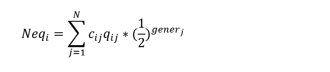
where N is the number of animals in the genomic base population, q~ij~ is the fraction relating the contribution of base population i to the total genetic value of the animal j, gener~j~ is the maximum number of generations between animal j and base population i, and c~i~j is the contribution of the genomic base animal j to base population i. So for example, a genotyped individual has one non-genotyped parent, hence c equals 0.50. The genotyped individual is linked to a specific base population only through one grandparent, hence q is 0.25.

11.3.3. Auto-similarity to another base population

The second statistic is the extent to which the same genotype information was used for a pair of base populations, which we call auto-similarity of one base population to another. To illustrate the concept, imagine 24 balls, 8 red, 8 blue and 8 orange. The balls are placed in two bowls, so the first bowl contains 5 red and 4 blue balls. The second contains the remaining 3 red, 4 blue and 8 orange. The similarity of bowl one to bowl two is 3 red + 4 blue over 9 balls is 0.78. The similarity of the second bowl to the first one is 3 red + 4 blue over 15 balls is 0.47. The colors in the illustration are genotyped animals and the bowls are base populations. So auto-similarity of base population i to j (AS~i to j~) is calculated as:

where q~ik~ and q~jk~ and c~ik~ are defined as q~ij~ and c~ij~ in Chapter 11.3.2.. An AS~i to j~ of 0 means that genotype information available to two base populations is independent. A value of 1 means that genotype information available is identical.

11.3.4. Number of generations between pedigree and genomic base populations

The third statistic is the weighted average number of generations between base animals in a base population and the genomic base population. It is calculated as:

where q~ij~, c~ij~ and gener~j~ are defined as above. delta~Gener~ differentiates between many remote genotyped descendants and fewer proximate ones for a given Neq.

11.3.5. Syntax

PEDFILE <file name> !Groups 1.0 !DiagBasePop

Qualifier: !DiagBasePop The qualifier !DiagBasePop can be used to specify that additional statistics on the suitability of base populations for use as genetic groups or metafounders. The !DiagBasePop is currently only available for the hpblup solver.

11.3.6. Associated output files

Output file	Description
DiagBasePop.log	Summary of diagnostics
DBP_DescriptiveStats.log	Descriptive statistics of base populations
DBP_EquivalentNrBaseIndiv.log	Equivalent number of genotyped individuals in base population
DBP_AutoSimilarity.log	Auto-similarity of each base population with other base populations
DBP_WeightedNrGenerations.log	Number of generations between pedigree and genomic base populations

12. Validation studies with MiXBLUP

Estimated breeding values (EBV) are used to identify the best individuals to become the parents of the next generation. The implicit assumption is that EBV are a reasonable prediction of performance of future progeny. BLUP evaluations to estimate breeding values often span many generations. Statistical model and components of variance and covariance among traits may have been suitable for earlier generations, but to what extent do EBV of the current generation predict the performance of progeny well? This is explored in validation studies.

1.1 General

It is good management practice to do validation studies regularly. In practice, validation studies are quite cumbersome to do, involve a lot of manual work and are prone to making mistakes. This makes it difficult to compare results between validation studies. MiXValidate has been designed to facilitate validation studies that are easy to do and transparent to interpret. MiXValidate creates a partial dataset given the validation individuals and the genetic effect to validate. It verifies that the list of validation individuals does not contain multiple generations. It estimates breeding values for the partial dataset and for the full dataset. It calculates validation statistics that are well-defined. Finally, it displays the amount of information that is available for validating the EBV and it leaves out validation individuals that do not have sufficient data available for validation.

12.1. Validation individuals

MiXValidate supports two types of validation studies. Parent validation focuses on how well parent EBV predict progeny performance. Individual validation checks how well EBV predict future performance of the individual itself. Parent validation can be done for either sires or dams. The user provides a file with validation individuals. This is a text file with just a list of original IDs, one ID per line. Validation individuals have to be from a single generation. MiXValidate gives a warning if more than one generation of a family is present among the validation individuals. The youngest individual from such a family will have more data removed for validation than other validation individuals, thus affecting the validation statistics.

12.2. Validation effect

There are traits that are affected by the genotype of other individuals, in addition to the genotype of the individual itself. For example, daily gain of piglets in the first weeks of their life is also determined by the genotype of the dam. Social behavior of pen mates affects the growth of individuals, in addition to their own genotype. These are referred to as indirect genetic effects and direct genetic effects, respectively. The process of creating the partial dataset is completely dependent on which genetic effect needs to be validated. Data records are omitted based on the field in the data file with the validation effect. A trait with a statistical model with direct and indirect genetic effects therefore needs two separate MiXValidate analyses for validation: one for the direct genetic effect as validation effect and one for the indirect genetic effect as validation effect.

12.3. Creating partial dataset

The idea behind creating the partial dataset is to create a dataset that reflects the situation at the point of selection for breeding or further testing. Any performance records on relatives collected after selection of the individual should be removed. The common practice to use a specific date after which all data records are omitted, only works well in the case of non-overlapping generations. With individual validation, MiXValidate removes data records of validation individuals and their siblings, and of descendants of these two groups. With parent validation, MiXValidate removes data records of progeny of validation individuals, descendants of this progeny and descendants of siblings of validation individuals. If the user specifies to remove data records of validation individuals, then these will be removed, as well as data records of siblings of validation individuals. The above can be applied to any genetic effect as validation effect (Table 1).

Table 1. Type of data records and type of removal in partial dataset

Validation Effect	Direct	Direct	Maternal	Maternal	Maternal	Maternal
Validation Type	Parent	Individual	Parent	Parent	Individual	Individual
Data field	Direct	Direct	Maternal	Direct	Maternal	Direct
Validation Individual	X1	X2	X1	-	X2	-
Siblings^a^	X1	X3	X1	-	X3	-
Progeny^b^	X2	X3	X2	X3	X3	X3
Descendants^c^	X3	X3	X3	X3	X3	X3

^a^ Siblings of validation individuals
^b^ Progeny of validation individuals
^c^ Descendants of progeny or siblings of validation individuals
X1 data records are removed if !ValNoOwnPerf is specified
X2 data records are removed and removed records are used for validation statistics
X3 data records are removed and removed records are not used for validation statistics

Data records of descendants are removed to allow the user to do validation studies retrospectively, so in any generation before the current generation. Descendants are not included in the validation statistics. The user can also specify a list of individuals for which all data records should be removed. MiXValidate will not remove any additional records in the partial data. It can be used for example to use a fixed date by adding all individuals with a data record after the date to the remove list.

12.4. Types of validation

MiXValidate presents validation statistics of two types of forward validation: LR method (Legarra and Reverter, 2018) and adjusted-phenotype validation (Mäntysaari et al., 2010). The LR method compares solutions of validation individuals from evaluation of the partial data with the corresponding solutions from evaluation of the full data. Adjusted-phenotype validation compares solutions of validation individuals from evaluation of the partial data with omitted adjusted phenotypes. Adjusted-phenotype validation is implemented for direct genetic effects only, for now.

12.5. Command-line syntax

The recommended way to call MiXBLUP for a validation study is:

MiXBLUP.exe val -i <instruction file>

The old syntax is now deprecated but still supported:

MiXValidate.exe <instruction file>

12.6. Syntax

Starting point for the instruction file for MiXValidate is the MiXBLUP instruction file of the routine evaluation. A new section VALIDATION needs to be added and the qualifiers !YieldDev and !HeritabFile need to be added to the SOLVING section.

SOLVING
[...]
!YieldDev
!HeritabFile <name of file with heritability per trait>
VALIDATION
!ValList <name of file with validation individuals>
[!ValEffect <field name genetic effect to validate>]
[!ValParent <sire | dam>]
[!ValNoOwnPerf]
[!ValRemoveList <name of file with individuals to remove in partial data>]
[!ValMinRec <n>]
[!ValSolutions <solutions file>]

Qualifiers:

!ValList <name file> The !ValList qualifier is mandatory and specifies the name of the file with validation individuals. The file contains a record for each validation individual with only the ID of the individual.

!ValEffect <validation effect name> The !ValEffect qualifier is optional and specifies the genetic effect to validate. Default is the direct genetic effect.

!ValParent <sire | dam> The !ValParent qualifier is optional and specifies that parent validation will be used and for which parent. If the !ValParent qualifier is omitted, then individual validation will be used. If the !ValParent qualifier is used without a setting, then sire validation will be used.

!ValNoOwnPerf The !ValNoOwnPerf qualifier is optional and only has a meaning in the context of parent validation. It specifies that data records of validation individuals and their siblings will also be removed in the partial data.

!ValRemoveList <file with individuals to remove in partial data> The !ValRemoveList qualifier is optional and causes MiXValidate to remove ONLY data records of the individuals in the specified file, so no additional data records are removed.

!ValMinRec <n> The qualifier !ValMinRec is optional and specifies the minimum number of data records available for a validation individual to be included in the validation statistics. This minimum number applies to own performance in case of individual validation and progeny records in case of parent validation. Records of other descendants and siblings of validation individuals and their descendants do not count towards this minimum number. The default minimum number is 1.

!ValSolutions <name file> The qualifier !ValSolutions is optional and specifies the solutions file to use for validation. !ValSolutions is not needed in most cases, but it can be used to validate an index of all EBV in the evaluation, for example. The default is the default MiXBLUP file with genetic effect solutions (Solani.out or Solani.txt).

!YieldDev The qualifier !YieldDev is mandatory to enable adjusted-phenotype validation.

!HeritabFile <file with direct heritability per trait> The qualifier !HeritabFile is required for adjusted-phenotype validation to get realized prediction accuracies. The file contains a line for each trait. A line consists of trait name (case-sensitive) and direct heritability.

12.7. Validation statistics

Validation statistics can be found in MiXBLUP.log. The first table gives an overview of the amount of data available for validation. The example (Figure 1) is taken from a parent validation study, using dams, of a maternal genetic effect that was only fitted for trait1.

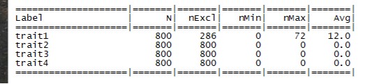
Figure 1. Overview of data available for validation of a maternal genetic effect

label	Field name of trait as specified in MiXValidate instruction file
N	Number of validation individuals
nExcl	Number of validation individuals excluded from calculation of validation statistics because of insufficient number of data records
nMin	Lowest number of data records for a validation individual
nMax	Highest number of data records for a validation individual
Avg	Average number of data records per validation individual

For individual validation, the number of data records is always on the individual itself only. For parent validation, it is the number of data records across progeny. In the example, validation individuals consisted of all dams in a generation. Of the 800 dams, 800 – 286 = 514 individuals had progeny appearing in the maternal genetic effect field of a data record, so progeny that were a dam, too. The number of data record per validation individual varied from 0 to 72 with an average of 12. A validation study using the same validation individuals and the same data records, but for the direct genetic effect gives a different table (Figure 2).

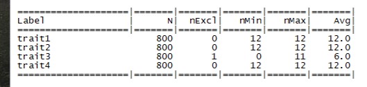
Figure 2. Overview of data available for validation of a direct genetic effect Validation statistics are presented in two or three tables, depending on the validation effect. The first table shows LR validation statistics only for included validation individuals. The last table show LR validation statistics for all validation individuals (Figure 3 and Figure 4).

Figure 3. Validation statistics for a maternal genetic effect The explanation of columns in these tables is as follows.

Solution	Combination of validation effect and trait name
n	Number of validation individuals included in calculations
intercept	Intercept of regressing solutions from full data (W) on solutions of partial data (P)
slope W on P	Slope of regressing solutions from full data (W) on solutions of partial data (P)
correlation	Pearson correlation between solutions from full data and solutions of partial data
level bias	Average of solutions from full data minus average of solutions from partial data
pred accuracy	Covariance between solutions from full data and solutions of partial data divided by genetic standard deviation among validation individuals.

The genetic standard deviation among validation individuals is estimated as the square root of (1-F~VI~)*var~A~, with F~VI~ the average inbreeding coefficient among validation animals and var~A~ the additive genetic variance that applies to the combination of validation effect and trait.

For validation studies of a direct genetic effect, the second table shows the adjusted-phenotype validation statistics (Figure 4).

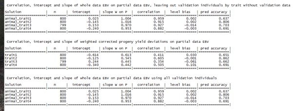
Figure 4. Validation statistics for a direct genetic effect.

The explanation of columns in the second table is as follows.

Solution	Combination of validation effect and trait name
n	Number of validation individuals included in calculations
intercept	Intercept of weighted regression of adjusted phenotypes from full data (W) on solutions of partial data (P)
slope W on P	Slope of weighted regression of adjusted phenotypes from full data (W) on solutions of partial data (P)
correlation	Weighted Pearson correlation between adjusted phenotypes from full data and solutions of partial data
level bias	Average of adjusted phenotypes from full data minus average of solutions from partial data
pred accuracy	Weighted correlation between adjusted phenotypes from full data and solutions of partial data divided by the expected prediction accuracy.

The expected prediction accuracy is calculated as the square root of N~prog~ * h^2^ /(N~prog~ * h^2^ + 4 – h^2^) for parent validation or the square root of h^2^ for individual validation, where N~prog~ is the average number of progeny records and h~2~ is the heritability of the combination of validation effect and trait, read from the file specified with !HeritabFile.

Adjusted phenotypes are obtained from the evaluation of the full data set and are the sum of genetic effects and the residual effect. The expectation of intercept and level bias is zero for LR validation if a suitable genetic base is used. A suitable genetic base consists of a number of high-reliability males at least two generation before the validation individuals. This can be done with !BaseAnimalsZero <file> in the SOLVING section. The expectation for slope is 1.0 for LR validation. For adjusted-phenotype validation, it is 0.5 for parent validation and 1.0 for individual validation. The realized prediction accuracy is an estimate of the average accuracy of estimated breeding values of validation individuals from the partial data. Note that this different from the calculated accuracy of estimated breeding values from the inverse coefficient matrix or approximations thereof (!Reliability). The latter is a relative measure of the amount of information available to estimate the breeding value assuming that the model and variance components are appropriate and that there is no confounding of effects. Note that this evaluation is based on the assumption that the accuracy (or reliability) of the EBV of validation individuals from the partial dataset is non-zero and more or less the same across validation animals. The realized prediction accuracy is an estimate of the average of this accuracy across validation individuals. It is advised not to include individuals with a much lower accuracy of the partial EBV in the group of validation individuals. Avoid parent-offspring pairs among the validation individuals for this reason.

12.8. Associated output files

Output file	Description
MiXBLUP.log	Contains the summary tables of validation statistics
LogValidationData.txt	For each validation individual by trait: number of data records, EBV partial & EBV whole

13. Indirect prediction

For an individual that is genotyped, but does not have a phenotype or progeny with a phenotype yet, each genomic estimated breeding value (GEBV) is just a function of SNP marker genotypes, SNP marker effects and the average polygenic estimated breeding value of its parents. There is limited benefit of solving equations for these animals iteratively. These GEBV can be predicted indirectly as a separate step after the routine genetic evaluation.

13.1. General

In some breeding programs, there is a constant influx of newly genotyped young individuals, but there are only a limited number of routine genetic evaluations in a year. Indirect prediction of their GEBV avoids having to run the full genetic evaluation multiple times. In other breeding programs, there may be a large number of genotyped individuals that will never have a phenotype or progeny with a phenotype. Using indirect prediction for these individuals reduces the size of the genetic evaluation and saves computing time and resources. Indirect prediction is a feature of the hpblup solver.

13.2. Indirectly predicting genomic estimated breeding values

13.2.1. General

If indirect prediction is used to predict GEBV of individuals without phenotypes or progeny with phenotypes, then these individuals are not included in the routine genetic evaluation. After the routine genetic evaluation is completed, the user provides a pedigree file and a genotype file that contain individuals in the evaluation and individuals excluded from the routine genetic evaluation. MiXBLUP identifies the latter group of individuals in the pedigree and genotype file and predicts GEBV for these individuals indirectly.

13.2.2. Supported evaluations

Indirectly predicting GEBV is only supported when using the hpblup solver and either ssSNPBLUP or ssGBLUP applying the Ta or Tac decomposition of G. MiXBLUP will verify that the routine genetic evaluation is suitable for indirect prediction. If the routine genetic evaluation is unsuitable, it will result in a fatal error.

13.2.3. Syntax

The recommended syntax for calling MiXBLUP for indirect prediction is:

MiXBLUP pred -p <pedigree file> -g <genotype file>

The old syntax is still supported:

MiXPred.exe -p <pedigree file> -g <genotype file>

13.2.4. Output files

The file with the solutions of the routine genetic evaluation is renamed to Solani_old.out. The solutions of routine genetic evaluation and those of indirect prediction are written to Solani.out.

14. Running MiXBLUP

This chapter describes practical issues when analyzing data with MiXBLUP.

14.1. Starting a MiXBLUP evaluation

Solving mixed model equations using MiXBLUP involves execution of several programs. The main executable is MiXBLUP.exe. This is the parser and it either calls the MiX99 executables dataprocessor.exe, solver.exe or reliabilities.exe, or it calls one of the hpblup executables hpblup.exe or hpblup_gpu.exe. For calculation of a genomic relationship matrix, MiXBLUP calls calc_grm.exe.

The recommended way to call MiXBLUP for breeding value estimation is:

MiXBLUP.exe blup -i <name instruction file>

Calling MiXBLUP without any arguments prints a help message (also available with the “--help” flag). Each flag under the new syntax has a long and a short version, long versions are always preceded by two dashes and short versions by a single dash. The user may choose the long versions for readability and documentation or the short ones for brevity and reduced typing.

Table with flag options:

Purpose	Command	Long flag	Short flag	Usage
EBV calculation	blup	--instruction	-i	Instruction file
Reliability	rel
Validation	val
Indirect Prediction	pred	--pedigree	-p	Pedigree file
		--genotype	-g	Genotype file
	any	--debug	-D	Debug options (s t m l)

The old syntax to call MiXBLUP is deprecated, but still available:

MiXBLUP.exe <name instruction file>

14.2. Choosing a breeding value evaluation or a reliability calculation

MiXBLUP either estimates breeding values, using either the default or the hpblup solver, or calculates approximate reliabilities, using reliabilities.exe. The type of analysis is controlled with the !RELIABILITY qualifier in the SOLVING section in the instruction file. If it is specified, a reliabilities calculation is started. See Chapter 9. for the additional changes in the instruction file when a reliabilities analysis is required. By default, a breeding value analysis is started. The hpblup solver can be called with !hpblup in the SOLVING section (see Chapter 8.).

14.3. A breeding value analysis with previous solutions as starting values

In case of large evaluations of breeding values, there may be a substantial saving in time to convergence of 10-30% by using the previous solutions as starting values for the current evaluation. This is activated by specifying the !RESTART qualifier or the !STARTVAL_CHECK qualifier in the SOLVING section. It does not have an effect on a reliabilities analysis. For the MiX99 solver, the only additional file necessary for using previous solutions is the Solunf file. If !RESTART is specified, MiXBLUP renames the file Solunf to Solold. If the file Solold is present, the preprocessor dataprocessor will create a file Solvec. This file will be used to initialise the solution vector of the mixed-model equations before the start of the iteration process (in solver). If any of the effects in the statistical model has been defined with field type A (alphanumerical labels), then the file Code.inp of the previous analysis must be present, too. The file Code_index.inp of a previous analysis is not used for a restart. For the hpblup solver, it is better to use !STARTVAL_CHECK instead of !RESTART. Additional files needed are startval_mixblup.new (in case the pedigree contains multiple base populations) or solutions_mixblup.dat (pedigree contains a single base population). MiXBLUP renames these files to startval_mixblup.dat. This file is read by the hpblup solver for initializing the solutions vector. The file hpCodes.bin is also needed as it contains the key between original and coded labels.

14.4. Monitoring and checking the process

When developing new analyses, it may be useful to monitor the progress of the analysis. This can be specified with “-D s” on the command line, for example

MiXBLUP blup -i TestRun.inp -D s

The output of the --debug or -D option is written to the screen log. Useful debug options:

-D s The debug option s provides more detail on the stage of the evaluation.

-D t The debug option t provides more detail on the run time of the various stages of the evaluation.

-D m The debug option m provides more detail on the memory use of the various stages of the evaluation.

-D l The debug option l (lowercase L) provides more detail on the current host, the license host, the type of license, the path to the license, and the end date of the license.

After the run is finished, it is worth to look through the various log-files. For the MiX99 solver, check ERMcalc_grm.log, dataprocessor.log and solver.log. For the hpblup solver, check ERMcalc_grm.log, hpblup.log and log_hpblup.dat. In MiXBLUP.log some information is given about pre- and post-processing of the data. It also lists error messages, if any. If all programs have run successfully, it is worth to check solver.log for the MiX99 solver or hpblup.log and convergence.dat for the hpblup solver, to see how the convergence was reached. In cases with poor convergence, it will give a warning and some model checking may be appropriate. When reliabilities are calculated, one can check the reliabilities.log, or reliabilities_direct.log and reliabilities_indirect.log when reliabilities are calculated for both direct and indirect genetic effects, such as maternal genetic effects.

14.5. Interrupting a process of the kernel

The MiX99 solver can be interrupted by placing an empty file with file name STOP in the folder of the analysis. The hpblup solver can be interrupted by placing an empty file with file name stopiter or STOP in the folder of the analysis. After every iteration, both solvers check whether the stop file is present. If so, it will start producing the output files as if convergence had been attained, instead of the next iteration, and it will stop afterwards.

15. Decoding any file with coded class effect labels

MiXBLUP produces quite a range of internal files with information that might be useful for the user in specific cases. Internal files contain coded labels of class effects and need to be decoded to be useful.

15.1. General

The solver requires that labels of class effect levels are coded 1 to N. In order to make coding and decoding as efficiently as possible, the key to code and decode labels is stored in a binary file. Therefore MiXBLUP has tools to decode files instead of to decode files manually.

15.2. Decoding coded labels

15.2.1. General

The decoding tool can be used for either the MiX99 or the hpblup solver. It will detect which solver has been used. If both types of key exist in the folder, the user is asked which key to use. If neither key exists, an error is given. The tool can be used to decode individual coded labels, a file with coded labels created by the user or an internal file created by MiXBLUP.

15.2.2. Syntax

The tool to decode coded labels is called from the command line as:

Coded2Original.exe

If the tool identifies hpblup as the solver used, it will ask for the field name in the genetic evaluation of the coded labels to decode.

hpblup: the file hpCodes.bin wil be used for decoding What is the field name of IDs to be decoded (not case-sensitive)?

The solver hpblup has a separate key for each class effect. Genetic class effect levels (i.e. IDs) of indirect genetic effects are coded using the key of the direct genetic effect. The MiX99 solver just has a single key for all alphanumerical class effects.

MiX99: the file code.inp wil be used for decoding

15.2.3. Decoding individual coded class effect labels

For decoding (one or a few) individual class effect labels, answer ‘1’ to the question

Do you want to decode (1) individual IDs or (2) a file with coded IDs?

The user then specifies the codes to decode one by one and closes by entering code ‘0’, which closes the tool.

15.2.4. Decoding a file that contains coded class effect labels

For decoding (one or a few) individual class effect labels, answer ‘2’ to the question

Do you want to decode (1) individual IDs or (2) a file with coded IDs?

The user is then asked three more questions:

Enter name of file with IDs to convert:
Enter field number with coded IDs to decode:
Enter name of new file with decoded IDs:
The new file is the same as the existing file, except for the coded label replaced with the original label.